Mean Structure for Quantitative Predictors

Location and/or Scale Changes (Reading: Faraway (2005, 1st edition), 5.2)

Using the saving data and fit the model:

> savings <- read.table("savings.data")
> g <- lm(sav ~ p15 + p75 + inc + gro, data=savings)
> summary(g)

• The coefficient for income is rather small --- let's measure income in thousands of dollars instead and refit:

  > g <- lm(sav ~ p15 + p75 + I(inc/1000) + gro, data=savings)
  > summary(g)

  Coefficients:

              Estimate Std. Error t value Pr(>|t|)   

  (Intercept)  28.5666     7.3545   3.884 0.000334 ***

  p15          -0.4612     0.1446  -3.189 0.002602 **

  p75          -1.6916     1.0836  -1.561 0.125508   

  I(inc/1000)  -0.3368     0.9311  -0.362 0.719296   

  gro           0.4097     0.1962   2.088 0.042468 * 

  ---

  Signif. codes:  0 `***' 0.001 `**' 0.01 `*' 0.05 `.' 0.1 ` ' 1

   

  Residual standard error: 3.803 on 45 degrees of freedom

  Multiple R-Squared: 0.3385,     Adjusted R-squared: 0.2797

  F-statistic: 5.756 on 4 and 45 DF,  p-value: 0.0007902

  • Q: What changed and what stayed the same?

• Q: What will happen if you divide the response by 10.

One rather thorough approach to scaling is to convert all the variables to standard unit (mean=0 and variance=1) using the "scale" command:

> scsav <- data.frame(scale(savings))

> mean(scsav)

> cov(scsav)

> g <- lm(sav~., data=scsav)

> summary(g)

• As may be seen, the intercept is zero. This is because the regression plane always runs through the point of the averages, which (because of the centering) is now at the origin.

• Such scaling has the advantage of putting all the predictors and the response on a comparable scale, which makes comparisons simpler.

• It also allows the coefficients to be viewed as kind of partial correlation --- the values will always be between -1 and 1.

• It also avoids some numerical problems that can arise when variables are of very different scales.

• The downside of this scaling is that the regression coefficients now represent the effect of a one standard unit increase in the predictor on the response in standard units --- this might not always be easy to interpret.

Polynomial Regression (Reading: Faraway (2005, 1st edition), 7.2.2)

Let's see if we can use polynomial regression on the gro variable in the savings data:

> savings <- read.table("savings.data")
> plot(savings$gro, savings$sav)

• Q: Does this relationship look linear?

First fit a linear model:

> summary(lm(sav ~ gro, data=savings))

• p-value of gro is significant so move on to a quadratic term:

  > summary(lm(sav ~ gro + I(gro^2), data=savings))

  Coefficients:

              Estimate Std. Error t value Pr(>|t|)   

  (Intercept)  5.13038    1.43472   3.576 0.000821 ***

  gro          1.75752    0.53772   3.268 0.002026 **

  I(gro^2)    -0.09299    0.03612  -2.574 0.013262 * 

  ---

  Signif. codes:  0 `***' 0.001 `**' 0.01 `*' 0.05 `.' 0.1 ` ' 1

  Residual standard error: 4.079 on 47 degrees of freedom

  Multiple R-Squared: 0.205,      Adjusted R-squared: 0.1711

  F-statistic: 6.059 on 2 and 47 DF,  p-value: 0.004559

  • Again p-value of gro^2 is significant so move on to a cubic term:

    > summary(lm(sav ~ gro + I(gro^2) + I(gro^3), data=savings))

    Coefficients:

                  Estimate Std. Error t value Pr(>|t|) 

    (Intercept)  5.145e+00  2.199e+00   2.340   0.0237 *

    gro          1.746e+00  1.380e+00   1.265   0.2123 

    I(gro^2)    -9.097e-02  2.256e-01  -0.403   0.6886 

    I(gro^3)    -8.497e-05  9.374e-03  -0.009   0.9928 

    ---

    Signif. codes:  0 `***' 0.001 `**' 0.01 `*' 0.05 `.' 0.1 ` ' 1

    Residual standard error: 4.123 on 46 degrees of freedom

    Multiple R-Squared: 0.205,      Adjusted R-squared: 0.1531

    F-statistic: 3.953 on 3 and 46 DF,  p-value: 0.01369

    • p-value of gro^3 is not significant so stick with the quadratic.

    • Q: What do you notice about the other p-values?

    • Check that starting from a large model (including the fourth power) and working downwards gives the same result.

  • Q: Why do we find a quadratic model when the lab on transforming predictors found that the gro variable did not need transformation?

    　

To illustrate the point about the significance of lower order terms, suppose we transform gro variable by subtracting 10 and refit the quadratic model:

> savings <- data.frame(savings, mgro=savings$gro-10)

> summary(lm(sav~mgro+I(mgro^2), data=savings))

• We see that the quadratic term remains unchanged but the linear term is now insignificant.

• Since there is often no necessary importance to zero on a scale of measurement, there is no good reason to remove the linear term in this model but not in the previous version. No advantage would be gained.

You have to refit the model each time a term is removed. Orthogonal polynomials save some time in this process - the "poly()" function in R constructs these:

> g <- lm(sav ~ poly(gro,4), data=savings) # fit a 4th-order polynomial model

> summary(g)

• We can see that the correlation between the parameter estimates are zero.

• Q: Can you see how we come to the same conclusion as above with just this summary?

• We can verify the orthogonality of the model matrix when using orthogonal polynomials:

  > x <- model.matrix(g)

  > dimnames(x) <- list(NULL, c("intercept","power1","power2","power3","power4"))

  > round(t(x)%*%x, 3)

              intercept power1 power2 power3 power4

    intercept        50      0      0      0      0

    power1            0      1      0      0      0

    power2            0      0      1      0      0

    power3            0      0      0      1      0

    power4            0      0      0      0      1　

• We can also do multivariate polynomials as in:

  > summary(lm(sav ~ poly(gro,inc, degree=2), data=savings))

  Coefficients:

                                Estimate Std. Error t value Pr(>|t|)   

  (Intercept)                     9.9517     0.5626  17.688  < 2e-16 ***

  poly(gro, inc, degree = 2)1.0  20.2395     6.8359   2.961  0.00493 **

  poly(gro, inc, degree = 2)2.0  -3.0943     4.7410  -0.653  0.51737   

  poly(gro, inc, degree = 2)0.1  11.5943     4.6938   2.470  0.01746 * 

  poly(gro, inc, degree = 2)1.1 108.4028    60.7661   1.784  0.08133 . 

  poly(gro, inc, degree = 2)0.2  -5.2894     4.0883  -1.294  0.20249   

  ---

  Signif. codes:  0 '***' 0.001 '**' 0.01 '*' 0.05 '.' 0.1 ' ' 1

   

  Residual standard error: 3.82 on 44 degrees of freedom

  Multiple R-Squared: 0.3474,     Adjusted R-squared: 0.2733

  F-statistic: 4.685 on 5 and 44 DF,  p-value: 0.001627

Broken Stick Regression (Reading: Faraway (2005, 1st edition), 7.2.1)

• In the analysis of the savings data, we observed that there were two groups in the data

• We might want to fit a different model to the two parts.

Suppose we focus attention on just the p15 predictor for ease of presentation. We fit the two regression models depending on whether p15 is greater or less than 35%:

> g1 <- lm(sav~p15, data=savings, subset=(p15<35))
> g2 <- lm(sav~p15, data=savings, subset=(p15>35))
> plot(savings$p15, savings$sav, xlab="Pop'n under 15", ylab="savings rate")
> abline(v=35, lty=5)
> segments(20, g1$coef[1]+g1$coef[2]*20, 35, g1$coef[1]+g1$coef[2]*35)
> segments(48, g2$coef[1]+g2$coef[2]*48, 35, g2$coef[1]+g2$coef[2]*35)

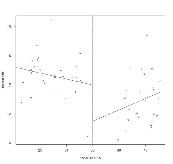
• A possible objection to this subsetted regression fit is that the two parts of the fit do not meet at the join.

• If we believe the fit should be continuous as the predictor varies, then this is unsatisfactory.

• One solution is to use broken line regression:

  > d <- function(x) ifelse(x<35, 0, 1)
  > gb <- lm(sav ~ p15+I((p15-35)*d(p15)), data=savings)
  > x <- seq(20, 48, by=1)
  > py <- gb$coef[1]+gb$coef[2]*x+gb$coef[3]*((x-35)*d(x))
  > lines(x, py, lty=2)

  

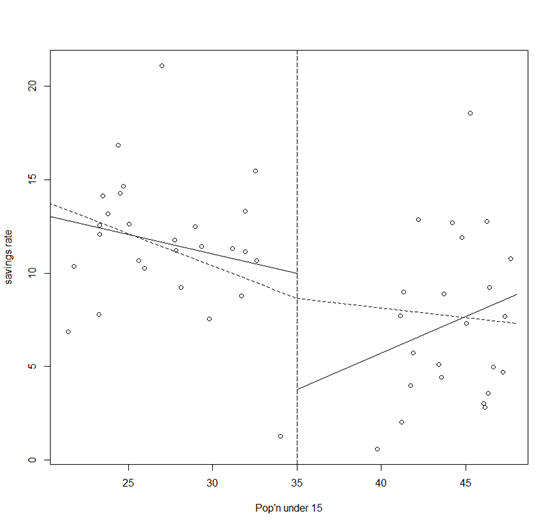
  • The two (dotted) lines now meet at 35 as shown in the plot.

  • The intercept of this model is the value of the response at the join.

  • We might question which fit is preferable in this particular instance.

    • For the high p15 countries, we see that the imposition of continuity causes a change in sign for the slope of the fit.

    • We might argue that the two groups of countries are so different and that there are so few countries in the middle region, that we might not want to impose continuity at all. 

Regression Spline (Reading: Faraway (2005, 1st edition), 7.2.3)

Let's see how the regression spline method perform on a constructed example.

• Suppose we know the true model is: 

y=sin³(2πx³)+ε,  ε~N(0, 0.01).

• The advantage of using simulated data is that we can see how close our methods come to the truth. We generate the data and display it in plots:

> funky <- function(x) sin(2*pi*x^3)^3
> x <- seq(0,1,by=0.01)
> y <- funky(x) + 0.1*rnorm(101)

> matplot(x,cbind(y,funky(x)),type="pl",ylab="y",pch=18,lty=1,main="True Model")

We see how an orthogonal polynomial bases of orders 4, 9, and 12 do in fitting this data:

> g4 <- lm(y~poly(x,4))

> g9 <- lm(y~poly(x,9))
> g12 <- lm(y~poly(x,12))
> matplot(x,cbind(y,g4$fit,g9$fit,g12$fit),type="plll",ylab="y",pch=18,lty=c(1,2,3),main="orthogonal polynomials")

• We see that order 4 is a clear lack-of-fit.

• Order 12 is much better although the fit is too wiggly in the first section and misses the point of inflection.

We now create the B-spline basis. You need to have three additional knots at the start and end to get the right basis. I have chosen to the knot locations to put more in regions of greater curvature. I have used 12 basis functions for comparability to the orthogonal polynomial fit.

> library(splines)

> knots <- c(0,0,0,0,0.2,0.4,0.5,0.6,0.7,0.8,0.85,0.9,1,1,1,1)
> bx <- splineDesign(knots,x)
> matplot(x,bx,type="l",main="B-spline basis functions")

> gs <- lm(y~bx)

> matplot(x,cbind(y,funky(x),gs$fit),type="pll",ylab="y",pch=18,lty=1,main="Spline fit")

The basis functions themselves are shown in the 3rd panel, while the fit itself appears in the 4th panel. We see that the fit comes very close to the truth. 

LOWESS and LOESS (Reading: Faraway (2006, 1st edition), 11.3)

Let's try to fit the data non-parametrically. For LOWESS and LOESS smoother, the key is to pick the window width well. The default choice (f=2/3 for LOWESS, which take 2/3 of the data, and span=3/4 for LOESS, which take 3/4 of the data) is not always good. Actually, it's criticized the default window width is too wide (resulting fitted line is too smooth). You should try different window widths and pick one which you think fit better. The LOWESS smoother in R:

> ls1 <- lowess(x, y, f=0.05)

> ls2 <- lowess(x, y, f=0.2)

> ls3 <- lowess(x, y, f=0.4)

> ls4 <- lowess(x, y, f=0.6)

> matplot(x,cbind(y,ls1$y,ls2$y,ls3$y,ls4$y),type="plll",ylab="y",pch=18,lty=c(1,2,3),main="LOWESS fit")

The LOESS smoother in R:

> loe1 <- loess(y~x, span=0.1)
> loe2 <- loess(y~x, span=0.3)
> loe3 <- loess(y~x, span=0.5)
> loe4 <- loess(y~x, span=0.7)

> matplot(x,cbind(y,loe1$fit,loe2$fit,loe3$fit,loe4$fit),type="pllll",ylab="y",pch=18,lty=c(1,2,3,4),main="LOESS fit")

It can be found from the plots that larger window width produces smoother line while smaller window width generates better fit.