The Longley dataset used in previous lab is a good example of collinearity:
> data(longley)
>
g <- lm(Employed ~ ., data=longley)
> summary(g)
Coefficients:
Estimate Std. Error t value Pr(>|t|)
(Intercept) -3.482e+03 8.904e+02 -3.911 0.003560 **
GNP.deflator 1.506e-02 8.492e-02 0.177 0.863141
GNP
-3.582e-02 3.349e-02 -1.070 0.312681
Unemployed -2.020e-02 4.884e-03 -4.136 0.002535 **
Armed.Forces -1.033e-02 2.143e-03 -4.822 0.000944 ***
Population -5.110e-02 2.261e-01 -0.226 0.826212
Year
1.829e+00 4.555e-01 4.016 0.003037 **
---
Signif. codes: 0 `***' 0.001 `**' 0.01 `*' 0.05 `.' 0.1
` ' 1
Residual standard error: 0.3049
on 9 degrees of freedom
Multiple R-Squared:
0.9955, Adjusted
R-squared: 0.9925
F-statistic: 330.3 on 6 and 9 DF, p-value: 4.984e-10
Recall that the response is number employed. Three of the predictors have large p-values but all are variables that might be expected to affect the response. Why aren't they significant? Check the correlation matrix first (rounding to 3 digits for convenience)
> round(cor(longley[,-7]),3)
GNP.deflator GNP
Unemployed Armed.Forces Population
Year
GNP.deflator
1.000 0.992
0.621
0.465
0.979 0.991
GNP
0.992 1.000
0.604
0.446
0.991 0.995
Unemployed
0.621 0.604
1.000
-0.177
0.687 0.668
Armed.Forces
0.465 0.446
-0.177
1.000
0.364 0.417
Population
0.979 0.991
0.687
0.364
1.000 0.994
Year 0.991 0.995 0.668 0.417 0.994 1.000
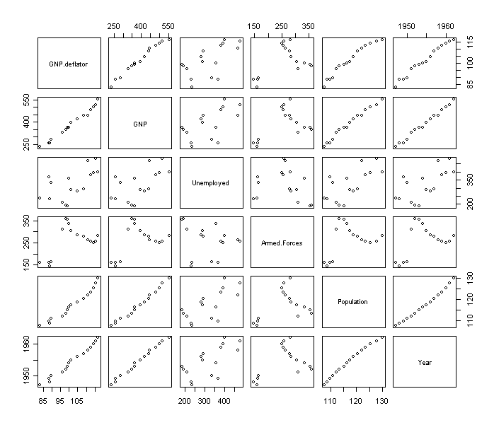
There are several large pairwise correlations. It can be also revealed from their pairwise scatter plots:
> x <- as.matrix(longley[,-7])
> pairs(x)
Now we check the eigen-decomposition:
>
e <- eigen( t(x) %*% x)
> e
$values
[1] 6.665299e+07 2.090730e+05 1.053550e+05 1.803976e+04 2.455730e+01 2.015117e+00
$vectors
[,1] [,2] [,3] [,4] [,5] [,6]
[1,] -0.04990131 0.06979071 -0.03416853 0.04265870 0.95653127 -0.2733126381
[2,] -0.19075418 0.72496814 -0.34330489 0.55402997 -0.07487553 0.0872940138
[3,] -0.15702286 0.62152746 0.56371985 -0.52067703 -0.00716578 0.0105568115
[4,] -0.12796016 0.10434859 -0.74630465 -0.64468394 -0.01222896 -0.0001122542
[5,] -0.05758090 0.03841364 -0.01095845 0.03583083 -0.28108541 -0.9564496276
[6,] -0.95748481 -0.26625145 0.07812474 0.05679111 -0.01522131 0.0526555591
> sqrt(e$value[1]/e$value)
[1] 1.00000 17.85504 25.15256 60.78472 1647.47771 5751.21560
There is a wide range in the eigenvalues and several condition numbers are large. This means that problems are being caused by more than just one linear combination. Now check out the variance inflation factors (VIF). For the first variable this is:
> summary(lm( x[,1] ~ x[,-1]))$r.squared
[1] 0.9926217
>
1/(1-0.9926217)
[1] 135.5326
which is large - the VIF for orthogonal predictors is 1. Here is a function to compute all the VIF's in one go:
> vif(x)
[1] 135.53244 1788.51348 33.61889 3.58893 399.15102 758.98060
There's definitely a lot of variance inflation! For example, we can interpret sqrt(1788)=42.28 as telling us that the standard error for GNP is 42 times larger than it would have been without collinearity. How can we get rid of this problem? One way is to throw out some of the variables. Examine the full correlation matrix above. Notice that variables 3 and 4 (Unemployed and Armed.Forces) do not have extremely large pairwise correlations with the other variables so we should keep them and focus on the others for candidates for removal:
> cor(x[,-c(3,4)])
GNP deflator GNP
Population Year
GNP
deflator 1.0000001 0.9915892 0.9791635
0.9911493
GNP 0.9915892 1.0000000 0.9910901 0.9952735
Population 0.9791635 0.9910901 1.0000001
0.9939529
Year
0.9911493 0.9952735 0.9939529 1.0000000
These four variables are strongly correlated with each other - any one of them could do the job of representing the others - we could pick year arbitrarily:
> summary(lm(Employed ~ Armed.Forces + Unemployed + Year, data=longley))
Coefficients:
Estimate Std. Error t value Pr(>|t|)
(Intercept) -1.797e+03 6.864e+01 -26.183 5.89e-12 ***
Armed.Forces -7.723e-03 1.837e-03 -4.204 0.00122 **
Unemployed -1.470e-02 1.671e-03 -8.793 1.41e-06 ***
Year
9.564e-01 3.553e-02 26.921 4.24e-12 ***
---
Signif. codes: 0 `***' 0.001 `**' 0.01 `*' 0.05 `.' 0.1
` ' 1
Residual standard error: 0.3321
on 12 degrees of freedom
Multiple R-Squared:
0.9928, Adjusted
R-squared: 0.9911
F-statistic: 555.2 on 3 and 12 DF, p-value: 3.916e-13
Compare this with the original fit - what do you find? We see that the fit is very similar but only three rather than six predictors are used.
One final point - extreme collinearity can cause problems in computing the estimates - look what happens when we use the direct formula for b-hat on the data with a 100 times larger scale change on first predictor:
>
xsc <- as.matrix(cbind(1, 100*x[,1], x[,2:6]))
> solve(t(xsc) %*% xsc) %*% t(xsc) %*%
longley$Employed
Error in solve.default(t(xsc) %*% xsc) : singular matrix `a' in solve
R, like most statistical packages, uses a more numerically stable method for computing the estimates in lm().
> lm(longley$Employed~xsc-1)
Call:
lm(formula = longley$Employed ~ xsc - 1)
Coefficients:
xsc xsc xscGNP xscUnemployed xscArmed.Forces
-3.482e+03 1.506e-04 -3.582e-02 -2.020e-02 -1.033e-02
xscPopulation xscYear
-5.110e-02 1.829e+00
We use the Longley data for this example:
> data(longley)
> longley # take a look
> x <- as.matrix(longley[,-7])
> y <- longley[,7]
First
we compute the eigen-decomposition for XTX
> e <-
eigen(t(x) %*% x)
Look at the eigenvalues:
> e$values
[1] 6.665299e+07 2.090730e+05 1.053550e+05 1.803976e+04 2.455730e+01 2.015117e+00
Look at the relative size - the first is big. Consider the first eigenvector (column) below:
> dimnames(e$vectors) <- list(c("GNP def","GNP","Unem","Armed","Popn","Year"),paste("EV",1:6))
> e$vectors
EV 1 EV 2 EV 3 EV 4 EV 5 EV 6
GNP def -0.04990131 0.06979071 -0.03416853 0.04265870 0.95653127 -0.2733126381
GNP -0.19075418 0.72496814 -0.34330489 0.55402997 -0.07487553 0.0872940138
Unem -0.15702286 0.62152746 0.56371985 -0.52067703 -0.00716578 0.0105568115
Armed -0.12796016 0.10434859 -0.74630465 -0.64468394 -0.01222896 -0.0001122542
Popn -0.05758090 0.03841364 -0.01095845 0.03583083 -0.28108541 -0.9564496276
Year -0.95748481 -0.26625145 0.07812474 0.05679111 -0.01522131 0.0526555591
The first eigenvector is dominated by Year (because the coefficient for Year in the 1st eigenvector is 0.95748481, which is much larger than other coefficients). Why is it? Now examining the X-matrix. What are the scales of the variables?
> x
GNP
deflator GNP Unemployed Armed Forces Population
Year
1947 83.0
234.289
235.6 159.0 107.608
1947
1948 88.5
259.426
232.5 145.6 108.632
1948
1949 88.2
258.054
368.2 161.6 109.773
1949
1950 89.5
284.599
335.1 165.0 110.929
1950
1951 96.2
328.975
209.9 309.9 112.075
1951
1952 98.1
346.999
193.2 359.4 113.270
1952
1953 99.0
365.385
187.0 354.7 115.094
1953
1954 100.0
363.112
357.8 335.0 116.219
1954
1955 101.2
397.469
290.4 304.8 117.388
1955
1956 104.6
419.180
282.2 285.7 118.734
1956
1957 108.4
442.769
293.6 279.8 120.445
1957
1958 110.8
444.546
468.1 263.7 121.950
1958
1959 112.6
482.704
381.3 255.2 123.366
1959
1960 114.2
502.601
393.1 251.4 125.368
1960
1961 115.7
518.173
480.6 257.2 127.852
1961
1962 116.9
554.894
400.7 282.7 130.081
1962
We see that these predictors have values in very different regions. The reason that Year stands up in the 1st principal component is because its values are much larger than others. It might make more sense to center the predictors before trying principal components. This is equivalent to doing principal components on the covariance matrix:
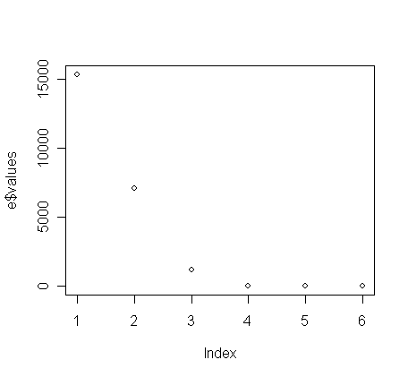
> e <- eigen(cov(x))
>
e$values
[1] 1.535852e+04 7.077406e+03
1.204409e+03 1.638766e+00 1.385096e-01 2.836721e-02
> plot(e$values
> dimnames(e$vectors) <- list(c("GNP def","GNP","Unem","Armed","Popn","Year"),paste("EV",1:6))
> e$vectors
EV 1 EV 2 EV 3 EV 4 EV 5 EV 6
GNP def -0.08247788 0.03437017 0.04184609 0.95671439 -0.269588027 0.047800192
GNP -0.75623528 0.31936977 0.55729097 -0.07632282 0.076772448 -0.061795997
Unem -0.62622375 -0.58026266 -0.52050055 -0.00739462 0.008954116 -0.009131889
Armed -0.15750866 0.74819438 -0.64438951 -0.01231829 -0.000605424 -0.002500043
Popn -0.05439163 0.01348608 0.03425705 -0.27999345 -0.927886716 0.237310015
Year -0.03717521 0.01184015 0.01853299 0.01642086 0.245711186 0.968241040
Can you give these P.C.'s (at least the first 3 P.C's) an interpretation based on the values in their eigenvectors? It can be observed that now GNP, Unemployed, and Armed Forces play the most important roles in the first three principal components, whose corresponding eigenvalues are large in contrast to rest eigenvalues. Why is it? Let's check the variances of these variables (see below). What have you observed and can you now understand why it happens?
> var(x)
GNP.deflator GNP
Unemployed Armed.Forces Population Year
GNP.deflator 116.45762 1063.6041 625.8666 349.0254 73.50300 50.92333
GNP
1063.60412 9879.3537
5612.4370
3088.0428 685.24094
470.97790
Unemployed 625.86663
5612.4370 8732.2343 -1153.7876 446.27415 297.30333
Armed.Forces 349.02538 3088.0428
-1153.7876
4843.0410 176.40981
138.24333
Population
73.50300 685.2409 446.2742 176.4098 48.38735 32.91740
Year 50.92333 470.9779 297.3033 138.2433 32.91740 22.66667
You can examine if Si var(xi) equals sum of eigenvalues.
> sum(diag(var(x)))
[1] 23642.14
> sum(e$values)
[1] 23642.14
Notice that the two values are identical. Why?
We can create the orthogonalized predictors --- the Z=XU operation as follows:
>
xpc <- x %*% e$vector
> round(cov(xpc),3)
EV 1 EV 2 EV 3 EV 4 EV 5 EV 6
EV 1 15358.52 0.000 0.000 0.000 0.000 0.000
EV 2 0.00 7077.406 0.000 0.000 0.000 0.000
EV 3 0.00 0.000 1204.409 0.000 0.000 0.000
EV 4 0.00 0.000 0.000 1.639 0.000 0.000
EV 5 0.00 0.000 0.000 0.000 0.139 0.000
EV 6 0.00 0.000 0.000 0.000 0.000 0.028
We can see that these new predictors, i.e. the principal components, are mutually orthogonal, and please note their variances are equal to their corresponding eigenvalues. Because these P.C.'s are obtained from non-centered X-matrix, they are not orthogonal to the constant term. You can check it by:
> round(summary(lm(y~xpc),cor=T)$cor,3)
To generate centered X-matrix, you can use:
>
xmean <- apply(x, 2, mean) # apply mean operation on the columns of x
>
cx <- sweep(x, 2, xmean) # sweep out mean on each columns of x
or equivalently use the command "cx <- scale(x, center=T, scale=F)".
We
now create the orthogonalized predictors using centered X-matrix:
>
cxpc <- cx %*% e$vector
Try to verify if the new predictors in cxpc are mutually orthogonal and orthogonal to the constant term in regression analysis:
> summary(lm(y~cxpc),cor=T)
Call:
lm(formula = y ~ xpc)
Residuals:
Min 1Q Median 3Q Max
-0.41011 -0.15767 -0.02816 0.10155 0.45539
Coefficients:
Estimate Std. Error t value Pr(>|t|)
(Intercept) -3.482e+03 8.904e+02 -3.911 0.00356 **
xpcEV 1 -2.510e-02 6.351e-04 -39.511 2.12e-11 ***
xpcEV 2 1.404e-02 9.356e-04 15.004 1.13e-07 ***
xpcEV 3 2.999e-02 2.268e-03 13.223 3.36e-07 ***
xpcEV 4 6.177e-02 6.149e-02 1.005 0.34137
xpcEV 5 4.899e-01 2.115e-01 2.316 0.04577 *
xpcEV 6 1.762e+00 4.673e-01 3.770 0.00441 **
---
Signif. codes: 0 '***' 0.001 '**' 0.01 '*' 0.05 '.' 0.1 ' ' 1
Residual standard error: 0.3049 on 9 degrees of freedom
Multiple R-Squared: 0.9955, Adjusted R-squared: 0.9925
F-statistic: 330.3 on 6 and 9 DF, p-value: 4.984e-10
Correlation of Coefficients:
(Intercept) xpcEV 1 xpcEV 2 xpcEV 3 xpcEV 4 xpcEV 5
xpcEV 1 0.00
xpcEV 2 0.00 0.00
xpcEV 3 0.00 0.00 0.00
xpcEV 4 0.00 0.00 0.00 0.00
xpcEV 5 -0.09 0.00 0.00 0.00 0.00
xpcEV 6 -1.00 0.00 0.00 0.00 0.00 0.00
In the fitted model, the b estimate, interpretation, and t-tests are much simplified because of the orthogonality between predictors.
Suppose you feel that the P.C.'s should not be influenced by the means and variances of the predictors. You may like to normalize these predictors to a same scale before trying principal component. This is equivalent to apply eigen-decomposition on its correlation matrix:
> e <- eigen(cor(x))
>
e$values
[1] 4.6033770958 1.1753404993 0.2034253724 0.0149282587 0.0025520658 0.0003767081
> sum(e$values)
[1] 6
Now, sum of eigenvalues = 6, which equals the number of predictors, why?
> dimnames(e$vectors) <- list(c("GNP def","GNP","Unem","Armed","Popn","Year"),paste("EV",1:6))
> e$vectors
EV 1 EV 2 EV 3 EV 4 EV 5 EV 6
GNP def 0.4618349 0.0578427677 0.1491199 0.792873559 -0.337937826 0.13518707
GNP 0.4615043 0.0532122862 0.2776823 -0.121621225 0.149573192 -0.81848082
Unem 0.3213167 -0.5955137627 -0.7283057 0.007645795 -0.009231961 -0.10745268
Armed 0.2015097 0.7981925480 -0.5616075 -0.077254979 -0.024252472 -0.01797096
Popn 0.4622794 -0.0455444698 0.1959846 -0.589744965 -0.548578173 0.31157087
Year 0.4649403 0.0006187884 0.1281157 -0.052286554 0.749542836 0.45040888
Can you give these P.C.'s (at least the first 3 P.C's) an interpretation based on the values in their eigenvectors?
One commonly used method of judging how many principal components are worth considering is to plot eigenvalues:
> plot(e$values, type="l", xlab="EV no.")
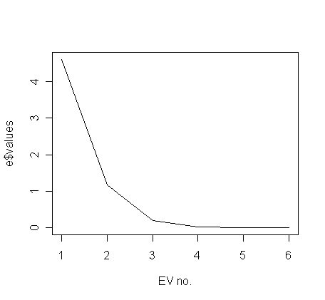
Often, the plot has a noticeable "elbow". Here the elbow is at about 3, which tells us that we need only consider the first two principle components. The first 2 P.C.'s explain about 94.9% (=0.650+0.299, see below) variation in the normalized X-matrix.
> round(e$value/sum(e$value),3)
[1] 0.650 0.299 0.051 0.000 0.000 0.000
One advantage of principal components is that it transforms the predictors to an orthogonal basis. To figure out the orthogonalized predictors for this data based on the eigen-decomposition for the correlation matrix of X, we must first normalize the data: The functions "scale()" is useful for doing this:
> nx <- scale(x) # the default is "center=Ture and scale=Ture"
Let us take a look of the covariance matrix of nx to examine whether it is normalized:
> cov(nx)
GNP.deflator GNP Unemployed Armed.Forces Population Year
GNP.deflator 1.0000000 0.9915892 0.6206334 0.4647442 0.9791634 0.9911492
GNP 0.9915892 1.0000000 0.6042609 0.4464368 0.9910901 0.9952735
Unemployed 0.6206334 0.6042609 1.0000000 -0.1774206 0.6865515 0.6682566
Armed.Forces 0.4647442 0.4464368 -0.1774206 1.0000000 0.3644163 0.4172451
Population 0.9791634 0.9910901 0.6865515 0.3644163 1.0000000 0.9939528
Year 0.9911492 0.9952735 0.6682566 0.4172451 0.9939528 1.0000000
We can now create the orthogonalized predictors, i.e., the P.C.'s, by;
> nxpc <- nx %*% e$vector
and fit:
> g <- lm(y~nxpc)
> summary(g)
Coefficients:
Estimate Std. Error t value Pr(>|t|)
(Intercept) 65.31700 0.07621 857.026 < 2e-16 ***
nxpcEV 1 1.56511 0.03669 42.662 1.07e-11 ***
nxpcEV 2 0.39183 0.07260 5.397 0.000435 ***
nxpcEV 3 -1.86039 0.17452 -10.660 2.10e-06
***
nxpcEV 4 0.35730 0.64423 0.555 0.592672
nxpcEV 5 -6.16983 1.55812 -3.960 0.003305 **
nxpcEV 6 6.96337 4.05550 1.717 0.120105
---
Signif. codes: 0 `***' 0.001 `**' 0.01 `*' 0.05 `.' 0.1
` ' 1
Residual standard error: 0.3049
on 9 degrees of freedom
Multiple R-Squared:
0.9955, Adjusted
R-squared: 0.9925
F-statistic: 330.3 on 6 and 9 DF, p-value: 4.984e-10
Notice that the p-values of the 4th and 6th P.C.'s are not significant while the 5th is. Because the directions of the eigenvectors are set successively in the greatest remaining direction of variation in the predictors, it's natural to expect that they are ordered in significance in predicting the response. However, there is no guarantee of this --- we see here that the 5th P.C. is significant while the 4th is not even though there is about six times greater variation in the 4th direction than the 5th. In this example, it hardly matters since most of the variation is explained by the earlier values, but look out for this effect in other dataset in the first few eigenvalues.
Check if all the predictors in model g are orthogonal:
> round(summary(g,cor=T)$cor,3)
(Intercept) nxpcEV 1 nxpcEV 2 nxpcEV 3 nxpcEV 4 nxpcEV 5 nxpcEV 6
(Intercept) 1 0 0 0 0 0 0
nxpcEV 1 0 1 0 0 0 0 0
nxpcEV 2 0 0 1 0 0 0 0
nxpcEV 3 0 0 0 1 0 0 0
nxpcEV 4 0 0 0 0 1 0 0
nxpcEV 5 0 0 0 0 0 1 0
nxpcEV 6 0 0 0 0 0 0 1
Notice now the P.C.'s are not only mutually orthogonal, they are also orthogonal to the constant term.
Principal
components are really only useful if we can interpret the meaning of the new
linear combinations. Look back at the first eigenvector - this is roughly a
linear combination of all the (normalized variables). Now plot each of the
variables as they change over time:
> par(mfrow=c(2,3))
> for(i
in 1:6) plot(longley[,6], longley[,i], type="l", xlab="Year",
ylab=names(longley)[i])
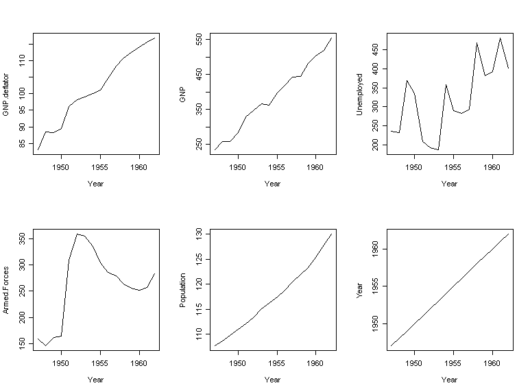
What do you notice? This suggests we identify the first principal component with a time trend effect. The second principal component is roughly a contrast between numbers unemployed and in the armed forces. Let's try fitting a regression with those two components:
> summary(lm(Employed ~ Year + I(Armed.Forces-Unemployed), data=longley))
Coefficients:
Estimate Std. Error t value Pr(>|t|)
(Intercept)
-1.391e+03 7.889e+01 -17.638
1.84e-10 ***
Year
7.454e-01 4.037e-02 18.463 1.04e-10 ***
I(Armed.Forces -
Unemployed) 4.119e-03 1.525e-03 2.701 0.0182 *
---
Signif. codes: 0 `***' 0.001 `**' 0.01 `*' 0.05 `.' 0.1
` ' 1
Residual standard error: 0.7178
on 13 degrees of freedom
Multiple R-Squared:
0.9638, Adjusted
R-squared: 0.9582
F-statistic: 173 on 2 and 13 DF, p-value: 4.285e-10
This approaches the fit of the full model and is easily interpretable. We need to do more work on the other principal components.
This example illustrates a typical use of principal components for regression. Some intuition is required to form new variables as combinations of older ones. It it works, a simplified and interpretable model is obtained, but it doesn't always work out that way.
We demonstrate the method on Longley data. You will need to load a library called "MASS" to help you on the analysis:
> data(longley)
> library(MASS)
> gr <- lm.ridge(Employed~., longley, lambda=seq(0,0.1,by=0.001)) # explore ridge trace in the region lÎ[0, 0.1]
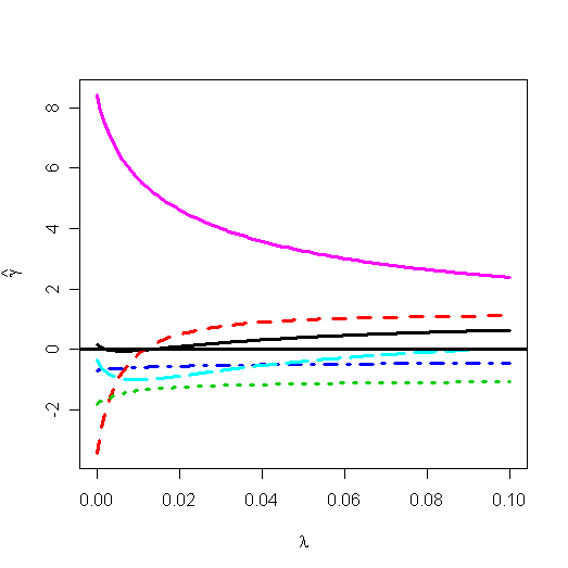
Let's plot the ridge trace:
> matplot(gr$lambda, t(gr$coef), type="l",
xlab=expression(lambda), ylab=expression(hat(gamma)), lwd=3)
> abline(h=0,
lwd=3)
You can find the ridge trace plot in graphic window. There are some
automate methods to select an appropriate l:
>
select(gr)
modified HKB estimator is
0.004275357
modified L-W estimator is 0.03229531
smallest
value of GCV at 0
> abline(v=0.004275357, lty=10, lwd=3) #
the HKB estimator
> abline(v=0.03229531, lty=11, lwd=3) # the L-W
estimator
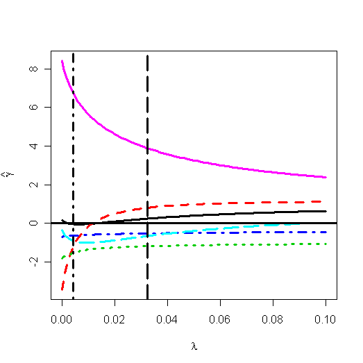
The Hoerl-Kennard (the originators of ridge regression) choice and L-W choice of l has been shown on the plot. I would prefer the value of 0.03. For this choice of l, the estimate of b is:
> gr$coef[, gr$lam == 0.03]
GNP.deflator
GNP Unemployed Armed.Forces
Population Year
0.2200496 0.7693585 -1.1894102
-0.5223393 -0.6861816 4.0064269
In contrast to the least squares estimates:
> gr$coef[, 1]
GNP.deflator
GNP Unemployed Armed.Forces
Population Year
0.1573796 -3.4471925 -1.8278860
-0.6962102 -0.3441972 8.4319716
Note that these values are based on centered and scaled predictors which explains the difference from previous fit. Consider the change in the coefficient for GNP. For the least squares fit, the effect of GNP is negative on the response --- number of people employed. This is counter-intuitive since we would expect the effect to be positive. The ridge estimate is positive, which is more in line with what we'd expect.