Testing for lack of fit (Reading: Faraway(2005, 1st edition), 6.3)

Variance known

• Using the same data as in the weighted least squares lab, we are going to test whether the model fitted in the previous lab is adequate.

• Because of the way the weights are defined, i.e., w_i=1/var(y_i), the known variance is implicitly equal to one (why?).

Let's first fit the weighted least square model.

> p <- read.table("phy.data", header=T) # read the data into R

> p # take a look of the data

> x <- p[,2]; y <- p[,3]; w <- 1/p[,4]^2 # extract variables and calculate weights

> g <- lm(y~x,weights=w) # fit a simple regression model with w as weights
> summary(g) # take a look of the fitted model

• Look at the high R² and the very small p-value for overall F-test

• Q: do you think the model is a good fit?

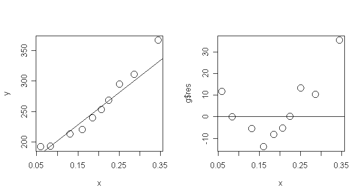
  • Now plot the data and the fitted regression line:
    > par(mfrow=c(1,2)) # split the graphic window into two

    > plot(x, y, cex=2) # draw the scatter plot of energy and crossx
    > abline(g$coef) # add the fitted line

    Now, let's also plot the residuals against crossx.

    > plot(x, g$res, cex=2); abline(0, 0) # draw scatter plot of residuals and crossx and add y=0 line

    

    • Q: What have you found from the plots?

    • Q: Whether or not the plots show that the fitted model is not good enough?

• Let's perform the test for lack of fit. Compute the test statistic and its p-value:

  > (8*1.657^2)/1 # test statistics = (n-p)*σ-hat²/σ²

  [1] 21.96519

  > 1-pchisq(21.96519, 8) # p-value of the test, the "pchisq" command returns the cdf value of a chi-square distribution

  [1] 0.004980762

  • Because the p-value is small, we conclude that there is a lack of fit.

  • Notice that although the original linear model had an R² of 94% and a very small overall F p-value, this in itself is not enough to conclude that this particular model fits.

Let us try to add a quadratic term, as suggested by the residual plot above, to the model and test again:

> g1 <- lm(y ~ x + I(x^2), weights=w) # fit a 2nd-order polynomial model
> summary(g1, cor=T) # take a look of the new fitted model

• The quadratic term is significant.

• The linear term becomes insignificant because of the strong collinearity between linear and quadratic terms.

  • However, it doesn't mean we should just drop the linear term. A better solution is to rescale the linear and quadratic terms so that they can be (almost) orthogonal.

• Let's perform the test for lack of fit on the new model.

  > (7*0.6788^2)/1  # calculate test statistic

  [1] 3.225386

  > 1-pchisq(3.225386, 7) # calculate p-value

  [1] 0.8633989

  • This time we cannot detect a lack of fit.

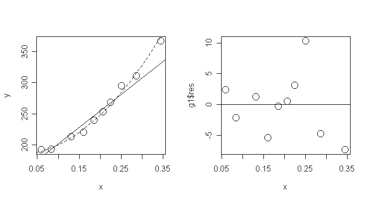
• Let's plot the fits of the two models and a residual plot under the new model:

  > plot(x, y, cex=2) # draw the scatter plot of energy and crossx
  > abline(g$coef) # add the fitted line of model g

  > xm <- seq(0.05, 0.35, 0.01); lines(xm, g1$coef[1]+g1$coef[2]*xm+g1$coef[3]*xm^2, lty=2) # add the fitted line of model g1

  > plot(x, g1$res, cex=2); abline(0, 0) # a residual plot under model g1

  

  • The quadratic model seems more appropriate than the linear model.

Variance unknown

• The data for this example consist of thirteen specimens of 90/10 Cu-Ni alloys with varying iron content in percent.

• The specimens were submerged in sear water for 60 days and the weight loss due to corrosion was recorded in units of milligrams per square decimeter per day.

> corrosion <- read.table("corrosion.data") # read the data into R

> corrosion # take a look of the data

• Notice that this is a data with some replication.

• Q: What is the source of variation in the replication?

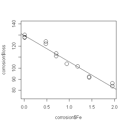
> g <- lm(loss ~ Fe, data=corrosion) # Fit a simple linear model with loss as response and Fe as predictor
> summary(g) # take a look of the fitted model

• Look at the high R² and the very small p-value for overall F-test.

• Q: Do you think this is a good fit?

  • Let's check the fit graphically:

    > plot(corrosion$Fe, corrosion$loss, ylim=c(80,140), cex=2) # draw the scatter plot of Fe and loss
    > abline(g$coef) # add the fitted line

    

    • Examine the plot and guess whether the test for lack of fit will be accepted or rejected.

To perform the test for lack of fit,

• We now fit a saturated model that reserves a parameter for each group of data with the same value of Fe.

• This is accomplished by declaring the predictor to be a factor in R. 

> ga <- lm(loss ~ factor(Fe), data=corrosion) # fit the saturated model, the "factor" command treats Fe as a qualitative predictor

> summary(ga) # take a look of the fitted saturated model

Notice that

• the saturated model has 7 parameters (including a constant term), which is equal to the number of distinct values of Fe.

• The residual standard error, 1.401, is a pure error estimate of true σ.

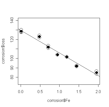
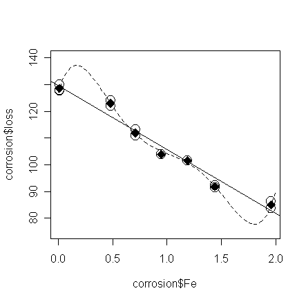
• The fitted values of the saturated model are the means in each group - put these on the plot:

  > points(corrosion$Fe, ga$fit, pch=18, cex=2) # add the means in each group to the plot

  

  • From the plot, do you think the model can pass the test for lack of fit?

• Here, let's calculate the SS and degrees of freedom for the pure error "by hand":

  > sum(ga$res^2) # calculate SS_p.e.

  [1] 11.78167

  > ga$df # the df_p.e.

  [1] 6

  > sum(g$res^2) # the RSS calculated from the model g

  [1] 102.8502

  We can put these values into the ANOVA table to calculate test statistic:

  	d.f.	SS	MS	F
  Residual	n-p  (11)	RSS  (102.8502)
  Lack of fit	n-p-dfp.e. (5)	RSS-SSp.e.	(RSS-SSp.e.)/(n-p-dfp.e. )	ratio of MS
  Pure error	dfp.e.  (6)	SSp.e.  (11.78167)	(SSp.e.)/(dfp.e.)

  And, now the test statistic:

  > ((102.8502-11.78167)/(11-6))/((11.78167/6)) # test statistic for lack of fit

  [1] 9.275615

  > 1-pf(9.275615, 5, 6) # the p-value

  [1] 0.008622849

• A slightly quicker way to get the same result:

  > anova(g, ga) # compute the ANOVA table for models g and ga

  Analysis of Variance Table

   

  Model 1: loss ~ Fe

  Model 2: loss ~ factor(Fe)

    Res.Df     RSS Df Sum of Sq      F   Pr(>F)  

  1     11 102.850                               

  2      6  11.782  5    91.069 9.2756 0.008623 **

  ---

  Signif. codes:  0 '***' 0.001 '**' 0.01 '*' 0.05 '.' 0.1 ' ' 1

  • The low p-value indicates that we must conclude that there is a lack of fit. 

Let's try to add more higher order polynomial terms one-by-one until the model pass the test for lack of fit:

> g1 <- lm(loss~Fe+I(Fe^2), data=corrosion) # fit a 2nd-order polynomial model
> anova(g1, ga) # compute the ANOVA table for models g1 and ga

> g2 <- lm(loss~Fe+I(Fe^2)+I(Fe^3), data=corrosion) # fit a 3rd-order polynomial model
> anova(g2, ga) # compute the ANOVA table for models g2 and ga

> g3 <- lm(loss~Fe+I(Fe^2)+I(Fe^3)+I(Fe^4), data=corrosion) # fit a 4th-order polynomial model
> anova(g3, ga) # compute the ANOVA table for models g3 and ga

> g4 <- lm(loss~Fe+I(Fe^2)+I(Fe^3)+I(Fe^4)+I(Fe^5), data=corrosion) # fit a 5th-order polynomial model
> anova(g4, ga) # compute the ANOVA table for models g4 and ga

Finally, the 5th-order polynomial model passes the test for lack of fit.

• This model is very close to the saturated model (the 6th-order polynomial model is a saturated model, why? Hint. count the number of parameters).

• Let's plot the fitted line of the 5-th order polynomial model and compare it with the straight line model:

  > grid <- seq(0, 2, length=50); lines(grid, predict(g4,data.frame(Fe=grid)), lty=2) # add the fitted line of the 5-th order model

  

  • Do you think the 5th order polynomial model is better than the straight line model?

    • We actually cannot explain why the corrosion loss should increase then decrease in the region 0<Fe<0.5, and decrease then increase in the region 1.5<Fe<2.0.

      • This is probably a consequence of over-fitting the data.

    • Because of the complexity of the model, the fitting on the observed Fe's is good, but the prediction on the region without observed Fe's becomes unstable.

    • In this case, we may want to stay with the straight line model and consider other reasons that may causes the lack of fit.

      • For example, you may want to find out whether the replicates are genuine.

      • Perhaps, the low pure error estimate can be explained by some correlation in the measurements.

      • The source of variation should also be examined.

        • For example, if the specimens with same Fe's are taken from different positions of a same unit, the pure error estimate does not include the variation between different units.

        • In the case, it is reasonable to get a pure error estimate lower than expected.

      • Other possible explanation is unmeasured predictors is causing the lack of fit.