Weighted least square (Reading: Faraway(2005, 1st edition), 6.2)

Look at here for a description of the data that we will use in this section.

• Q: Can you figure out from the description what weights should be used for the data and why?

> p <- read.table("phy.data", header=T) # note the extra argument to cope with not having row labels
> p # take a look of the data

Notice that

• The sd decreases along with the reduction of energy.

• Since the weights should be inversely proportional to the variance, this suggests that the weights should be set to 1/sd².

> x <- p[, 2] # extract the energy variable, the predictor
> y <- p[, 3] # extract the crossx variable, the response
> w <- 1/p[, 4]^2 # the weights
> g <- lm(y~x, weights=w) # fit the model with w as weights. "weights" adds as an option.
> summary(g) # take a look of the results

• We can test the significance of x by looking at the p-value from the coefficients table or by looking at the overall F-stat (they are equivalent, 11.16²=124.6, because this is a simple regression case).

• But, if we want to do it the hard way, we must construct the analysis of variance table by hand as follows:

  > sum(w*g$res*g$res) # the residual sum of squares

  [1] 21.95265

  > wm <- sum(w*y)/sum(w) # the weighted mean of y
  > sum(w*(y-wm)*(y-wm)) # the weighted total SS

  [1] 363.944

  > 363.944 - 21.95265 # the regression SS

  [1] 341.9914

  > (341.9914/1)/(21.95265/8) # the overall F statistic

  [1] 124.6287

Let's try fitting the regression without weights and see what the difference is:

> g1 <- lm(y~x) # fit the model without weights
> summary(g1) # take a look of the fitted model

• Compare the output to the summary of model g. Explain their differences.

  • R-square: why would g1 has a higher value than g?

  • σ-hat: Why are they so different? Do they estimate the same parameter?

  • residuals: Why are their ranges so different?

• The two fits can be compared:

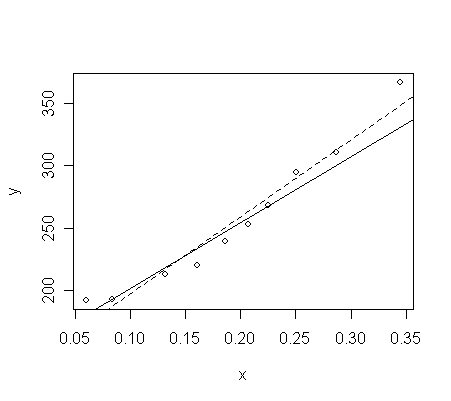
  > plot(x,y) # scatter plot of x and y
  > abline(g) # the fitted line of model g, solid line
  > abline(g1, lty=2) # the fitted line of model g2, dashed line

  

  • The un-weighted fit (dashed line) appears to fit the data better overall

  • But remember that for lower values of energy, the variance in the response is less.

  • The weighted fit (solid line) tries to catch these points with lower energy better than the others.

Weighted least square can be regarded as regressing sqrt(w_i)x_i on sqrt(w_i)y_i using ordinary least square:

> ym<-sqrt(w)*y # calculate sqrt(w_i)y_i
> xm<-sqrt(w)*x  # calculate sqrt(w_i)x_i

> g2 <- lm(ym~sqrt(w)+xm-1) # regressing sqrt(w_i)x_i on sqrt(w_i)y_i. "-1" drop the intercept.

• Note that the 1 column in X-matrix is replaced by sqrt(w_i)

> summary(g2) # take a look of the results

• Compare the output to the summary of model g. What quantities are different? Explain why.

• To get the correct overall F-test, we can use:

  > anova(lm(ym~sqrt(w)-1), g2) # the correct F-statistics

  Analysis of Variance Table

   

  Model 1: ym ~ sqrt(w) - 1

  Model 2: ym ~ sqrt(w) + xm - 1

    Res.Df    RSS Df Sum of Sq      F    Pr(>F)   

  1      9 363.94                                 

  2      8  21.95  1    341.99 124.63 3.710e-06 ***

  ---

  Signif. codes:  0 '***' 0.001 '**' 0.01 '*' 0.05 '.' 0.1 ' ' 1

  • You can use the two RSSs in the correct F-statistic to obtain the right R-square (How?)

Let's also check their residuals.

> print(g$res, digits=2) # the residuals of model g

> print(g2$res, digits=2) # the residuals of model g2

• Why are the two groups of residuals so different?

• Which residuals is y_i minus y_i-hat? Which residuals is sqrt(w_i)y_i minus sqrt(w_i)y_i-hat?

• Which residuals can be used to perform diagnostics (i.e., residual analysis) and to calculate σ-hat by directly taking sum of their squares?

• Let's find out the relationship between the two groups of residuals:

  > print(sqrt(w)*g$res, digits=2) # check if it equals residuals of model g2

       1      2      3      4      5      6      7      8      9     10

   2.082  1.131  1.476  0.013 -0.765 -1.368 -2.323 -0.924 -0.013  2.335