Correspondence Analysis (Reading: Faraway (2006), section 4.2)
When the test of independence for 2-way contingency table rejects the null, we know that the two variables are dependent. It might be nice to know where the dependence is coming from, i.e., how the two variables are associated. To study this, we can use a kind of residual analysis for 2-way contingency tables called correspondence analysis. It performs a singular value decomposition on a table formed by the Pearson residuals, which is obtained from a model corresponding to independence. Let us demonstrate by using the hair and eye color data discussed in the previous lab:
> haireye <- read.table("haireye.txt")
Now, let us fit a Poisson GLM containing only main effect terms (corresponding to independence) and extract its residuals:
> modc <- glm(y ~ hair + eye, family=poisson, haireye)
> z <- xtabs(residuals(modc,type="pearson")~hair+eye,haireye)
> svdz <- svd(z,2,2)
> leftsv <- svdz$u %*% diag(sqrt(svdz$d[1:2]))
> rightsv <- svdz$v %*% diag(sqrt(svdz$d[1:2]))
> ll <- 1.1*max(abs(rightsv), abs(leftsv)) #
because the distance between points in the correspondence plot is of interest,
it is important the plot is scaled so that the visual distance is
proportionately correct. Therefore, we will specify in next command the ranges
of x-axis and y-axis to be the value of ll
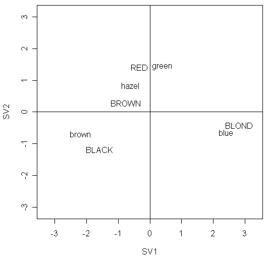
> plot(rbind(leftsv,rightsv),asp=1,xlim=c(-ll,ll),ylim=c(-ll,ll),xlab="SV1",ylab="SV2",type="n")
> abline(h=0,v=0)
> text(leftsv,dimnames(z)[[1]])
> text(rightsv,dimnames(z)[[2]])

In the plot, we should particularly pay attention to:
the points with large absolute values on x-axis or y-axis
its row or column profile is different.
for example, BLOND is far from the origin indicating the distribution of eye colors within this group of people is not typical
in contrast, BROWN is close to the origin, indicating an eye color distribution that is close to the overall average.
two points, one from the row variable of the table and one from the column variable, appear close together and far from the origin
the particular row-column combination of the two points associates with a large positive residual, which indicates a strong positive association
for example, the two points BLOND and blue shows that there are relatively more people with blond hair and blue eyes than would be expected under independence.
two points, one from the row variable and one from the column variable, situate diametrically apart on either side of the origin
the particular row-column combination of the two points associates with a large negative residual, which indicates a strong negative association
for example, the two points BLOND and brown shows that there are relatively fewer people with blond hair and brown eyes than would be expected under independence.
two points, both from the row variable or the column variable, are close together
the two rows (or two columns) have a similar pattern of association
in some cases, one might consider combining the two rows (or two columns)
for example, the two points hazel and green shows that people with hazel or green eyes have similar hair color distributions and we might choose to combine these two categories
two points, one from the row variable and one from the column variable, lie respectively near two lines y=ax and y=-(1/a)x for some a
the particular row-column combination of the two points has a relatively small residual because the components in the matrix expression for the relevant residual will tend to cancel
for example, the two points BLACK and hazel or the two points RED and brown