Two-Way Tables (Reading: Faraway (2006), section 4.1~4.2)
Two-by-Two Tables.
The data shown below were collected as part of a quality improvement study at a semiconductor factory.
| Quality | No Particles | Particles | Total |
| Good | 320 | 14 | 334 |
| Bad | 80 | 36 | 116 |
| Total | 400 | 50 | 450 |
A sample of wafers was drawn and cross-classified according to whether a particle was found on the die that produced the wafer and whether the wafer was good or bad. First, let us set up the data in a convenient form for analysis:
> y <-
c(320,14,80,36)
> particle <- gl(2,1,4,labels=c("no","yes"))
> quality <- gl(2,2,labels=c("good","bad"))
> wafer <- data.frame(y,particle,quality)
> wafer
y particle quality
1 320 no good
2 14 yes good
3 80 no bad
4 36 yes bad
We will need the data in this form with one observation per line for our model fitting, but usually we prefer to observe its table form:
> (ov <- xtabs(y ~ quality+particle))
particle
quality no yes
good 320 14
bad 80 36
The data might have arisen under several possible sampling schemes:
observe the manufacturing process for a certain period of time and observed 450 wafers Þ all the numbers are random Þ we could use a Poisson model
decide to sample 450 wafers Þ 450 is a fixed number and other numbers are random Þ we could use a multinomial model
select 400 wafers without particles and 50 wafers with particles Þ 400, 50, and 450 are fixed numbers and other numbers are random Þ we could use a binomial model
select 400 wafers without particles and 50 wafers with particles that also included, by design, 334 good wafers and 116 bad ones Þ 400, 50, 334, 116, and 450 are fixed numbers and other numbers are random Þ we could use a hypergeometric model
The main question of interest concerning these data is whether the presence of particles on the wafer affects the quality outcome. We shall see in the following that all four sampling schemes lead to exactly the same conclusion.
Sampling Scheme 1: Poisson Model.
Under sampling scheme 1, it would be natural to
view these outcomes, Yij,
1£i£I,
1£j£J, occurring at different rates,
lpij,
where l is an unknown value
of a size variable and pij
is the probability that a randomly selected subject falls in the
ijth cell. We can form
a Poisson
model for these rates, i.e., Yij~Poisson(lpij). Suppose
that we fit a Poisson GLM with only main effect terms:
>
modl <-
glm(y ~ particle+quality, poisson)
> summary(modl)
Call:
glm(formula = y ~ particle + quality, family = poisson)
Deviance Residuals:
1 2 3 4
1.324 -4.350 -2.370 5.266
Coefficients:
Estimate Std. Error z value Pr(>|z|)
(Intercept) 5.6934 0.0572 99.535 <2e-16 ***
particleyes -2.0794 0.1500 -13.863 <2e-16 ***
qualitybad -1.0576 0.1078 -9.813 <2e-16 ***
---
Signif. codes: 0 '***' 0.001 '**' 0.01 '*' 0.05 '.' 0.1 ' ' 1
(Dispersion parameter for poisson family taken to be 1)
Null deviance: 474.10 on 3 degrees of freedom
Residual deviance: 54.03 on 1 degrees of freedom
AIC: 83.774
Number of Fisher Scoring iterations: 5
Notice that:
the null model, which suggests all four outcomes occur at the same rate, does not fit because the deviance of 474.10 is very large for 3 degrees of freedom
the fitted model has a residual deviance of 54.03, which is clearly an improvement over the null model. An alternative goodness-of-fit measure is the Pearson X2:
> sum(residuals(modl,type="pearson")^2)
[1] 62.81231
we might also want to test the significance of the individual predictors. The null of the tests corresponds to the hypothesis of equivalent marginal proportions, i.e., p1+=p2+=...=pI+. or p+1=p+2=...=p+J. For the table, we could use the z-values in the output, but it is better to use the difference-in-deviance test:
> drop1(modl,test="Chi")
Single term deletions
Model:
y ~ particle + quality
Df Deviance AIC LRT Pr(Chi)
<none> 54.03 83.77
particle 1 363.91 391.66 309.88 < 2.2e-16 ***
quality 1 164.22 191.96 110.18 < 2.2e-16 ***
---
Signif. codes: 0 '***' 0.001 '**' 0.01 '*' 0.05 '.' 0.1 ' ' 1
We see that both predictors are significant relative to the fitted model. It suggests that the marginal proportions are not equivalent for both predictors.
by examining the coefficients, we see that wafers without particles occur at a significantly higher rate than wafer with particles because the estimated coefficient of particleyes is negative. Similarly, we see that good-quality wafers occur at a significantly higher rate than bad-quality wafers because the estimated coefficient of qualitybad is negative
the coefficients of a model containing only main effect terms are closely related to the marginal totals because the MLE of the rates m=(lpij) must satisfy XTy=XT(m-hat), where XTy is, in this example:
> (t(model.matrix(modl)) %*% y)[,]
(Intercept) particleyes qualitybad
450 50 116
So we see that the fitted values, m-hat, must be a function of marginal totals. The coding we use will determine exactly how the coefficients relate to the marginal totals. For example, consider the particle factor, which is coded as 0 and 1 for No Particle and Particle categories, respectively. Its fitted coefficient is:
> coef(modl)[2]
particleyes
-2.079442
> (coefparticle <- exp(c(0, coef(modl)[2])))
particleyes
1.000 0.125
> coefparticle/sum(coefparticle)
particleyes
0.8888889 0.1111111
We see that these are just the marginal proportions for the no particle wafers and particle wafers respectively:
> c(400, 50)/450
[1] 0.8888889 0.1111111
this model has a deviance of 54.03 on one degree of freedom and so does not fit the data. A Poisson GLM with only main effect terms corresponds to independent contingency tables, i.e., pij=pi+p+j. Because the model does not fit, we reject the hypothesis that good- or bad-quality outcomes would occur independently of whether a particle was found on the wafer.
the addition of an interaction term would saturate the model and so would have zero deviance and zero degrees of freedom. So, an hypothesis comparing the models with and without interaction would use a test statistic of 54.03 on one degree of freedom, which is exactly the goodness-of-fit test. The hypothesis of no interaction would be rejected --- the necessity to fit a Poisson GLM with interaction indicates that the two predictors are associated, i.e., dependent.
for each cells, the fitted values under the Poisson GLM with only main effect terms are:
> xtabs(fitted(modl) ~ quality+particle)
particle
quality no yes
good 296.88889 37.11111
bad 103.11111 12.88889
Notice that these fitted values form an independent contingency table because its odds-ratio is one:
> (296.88889*12.88889)/(103.11111*37.11111)
[1] 1.000000
Sampling Scheme 2: Multinomial Model.
> (pp <- prop.table( xtabs(y ~ particle)))
particle
no yes
0.8888889 0.1111111
> (qp <- prop.table( xtabs(y ~ quality)))
quality
good bad
0.7422222 0.2577778
and the fitted values, Yij-hat, of each cells under the independence hypothesis, i.e., pij=pi+p+j, are y++(pi+-hat)(p+j-hat):
> (fv <- outer(qp,pp)*450)
particle
quality no yes
good 296.8889 37.11111
bad 103.1111 12.88889
Notice that the fitted values are the same as that in the Poisson GLM with only main effect terms.
To test whether the fitted values are close to the observed values, we can compare this model against the saturated model, for which the MLE of cell counts are the observed values Yij. So, the log-likelihood-ratio test statistic for independence is 2SiSjYijlog[Yij/(Yij-hat)] [Note: it is because the log-likelihood of multinomial is SiSjYijlog(pij) ], which computes to:
> 2*sum(ov*log(ov/fv))
[1] 54.03045
This is the same deviance we observed in the Poisson model with only main effect terms. So, we see that the test for independence in the multinomial model coincides with the test for no interaction in the Poisson model. The latter test is easier to execute in R, so we shall usually take that approach.
One alternative to the deviance is the Pearson
X2 statistic SiSj[(Oij-Eij)2/Eij]:> sum( (ov-fv)^2/fv)
[1] 62.81231
which is also the same as that in the Poisson model with only main effect terms. We can apply Yates' continuity correction on the Pearson
X2 statistic, which gives superior results for small samples. This correction is implemented in:> prop.test(ov)
2-sample test for equality of proportions with continuity correction
data: ov
X-squared = 60.1239, df = 1, p-value = 8.907e-15
alternative hypothesis: two.sided
95 percent confidence interval:
0.1757321 0.3611252
sample estimates:
prop 1 prop 2
0.9580838 0.6896552
The
X2 statistic with continuity correction is 60.1239 for one degree of freedom, which clearly rejects the null, i.e., independence hypothesis.
Sampling Scheme 3: Binomial Model.
Under the sampling scheme 3, it would be natural to view the presence of the particle as a cause that affects the quality of wafer. In other words, we would view the variable quality as the response and the variable particle as a predictor. When the number of wafers with no particles is fixed at 400 and the number with particles at 50, we can use a binomial model for the response for both groups. To fit a binomial GLM to the response in R, we need to form a two-column matrix with the 1st column representing the number of "successes" and the 2nd column the number of "failures":
> (m <- matrix(y,nrow=2))
[,1] [,2]
[1,] 320 80
[2,] 14 36
Let us fit a binomial GLM that only contains a constant term, which suggests that the probability of the response is the same in both the particle and no particle group, i.e., a homogeneous model:
> modb <- glm(m ~ 1, family=binomial)
> summary(modb)
Call:
glm(formula = m ~ 1, family = binomial)
Deviance Residuals:
1 2
2.715 -6.831
Coefficients:
Estimate Std. Error z value Pr(>|z|)
(Intercept) 1.0576 0.1078 9.813 <2e-16 ***
---
Signif. codes: 0 '***' 0.001 '**' 0.01 '*' 0.05 '.' 0.1 ' ' 1
(Dispersion parameter for binomial family taken to be 1)
Null deviance: 54.03 on 1 degrees of freedom
Residual deviance: 54.03 on 1 degrees of freedom
AIC: 66.191
Number of Fisher Scoring iterations: 3
Notice that:
the deviance of the homogeneous binomial model, 54.03, is exactly the same as the deviance of the Poisson model containing only main effect terms
in other words, the hypothesis of homogeneity in the binomial GLM corresponds exactly to the hypothesis of independence in the Poisson GLM
Because either row or column marginal totals are fixed in this sampling scheme, the marginal totals in the table does not carry any useful information about the marginal proportions pi+ and p+j. Therefore, it does not make sense to test equivalence of marginal proportions for data obtained from the sampling scheme with fixed marginal totals.
Sampling Scheme 4: Hypergeometric Model.
Under the sampling scheme 4, if we fix any number in the table, say Y11, the remaining three numbers are completely determined because the row and column marginal totals are known. In the circumstance, the distribution of Y11 under the null hypothesis: pij=pi+p+j is a hypergeometric distribution. Because there is only a limited number of values which Y11 can possibly take, we can compute the total probability of all outcomes that are "more extreme" than the one observed. The total probability is then the p-value. The method is called Fisher's exact test:
> fisher.test(ov)
Fisher's Exact Test for Count Data
data: ov
p-value = 2.955e-13
alternative hypothesis: true odds ratio is not equal to 1
95 percent confidence interval:
5.090628 21.544071
sample estimates:
odds ratio
10.21331
Notice that:
the default takes as "more extreme" all Y11 with probabilities (under null) less than or equal to that of the observed Y11
the exact p-value, 2.955e-13, also suggests that the two variables quality and particle are not independent
the method estimates an odds ratio of 10.21331 with an exact confidence interval [5.090628, 21.544071]. Odd ratio is a measure of association for 2´2 table. We see that 10.21331 is much larger than one (odd-ratio=1 Û independence) and also the confidence interval does not contain one.
the sample odds ratio, which is (Y11Y22)/(Y12Y21), takes the value:
> (320*36)/(14*80)
[1] 10.28571
which is very close to 10.21331. An exact confidence interval can also be calculated as we see in the output of Fisher's exact test.
>
haireye <- read.table("haireye.txt")
> haireye
y eye hair
1 5 green BLACK
2 29 green BROWN
3 14 green RED
4 16 green BLOND
5 15 hazel BLACK
6 54 hazel BROWN
7 14 hazel RED
8 10 hazel BLOND
9 20 blue BLACK
10 84 blue BROWN
11 17 blue RED
12 94 blue BLOND
13 68 brown BLACK
14 119 brown BROWN
15 26 brown RED
16 7 brown BLOND
The data is more conveniently displayed using:
> (ct <- xtabs(y ~ hair + eye, haireye))
eye
hair blue brown green hazel
BLACK 20 68 5 15
BLOND 94 7 16 10
BROWN 84 119 29 54
RED 17 26 14 14
(Q: what information have you found by merely looking at the table?)
We can execute the usual Pearson's X2 test for independence as:
Call: xtabs(formula = y ~ hair + eye, data = haireye)
Number of cases in table: 592
Number of factors: 2
Test for independence of all factors:
Chisq = 138.29, df = 9, p-value = 2.325e-25
where
we see that hair and eye color are clearly not independent because an X2 of 138.29 on 9 degrees of freedom is way too large
9=(4-1)(4-1) is the degrees of freedom for the interaction between the two categorical variables.
Now, let us fit a Poisson GLM containing only main effect terms:
> modc <- glm(y ~ hair + eye, family=poisson, haireye)
> summary(modc)
Call:
glm(formula = y ~ hair + eye, family = poisson, data = haireye)
Deviance Residuals:
Min 1Q Median 3Q Max
-7.3263 -2.0646 -0.2120 1.2353 6.1724
Coefficients:
Estimate Std. Error z value Pr(>|z|)
(Intercept) 3.66926 0.11055 33.191 < 2e-16 ***
hairBLOND 0.16206 0.13089 1.238 0.21569
hairBROWN 0.97386 0.11294 8.623 < 2e-16 ***
hairRED -0.41945 0.15279 -2.745 0.00604 **
eyebrown 0.02299 0.09590 0.240 0.81054
eyegreen -1.21175 0.14239 -8.510 < 2e-16 ***
eyehazel -0.83804 0.12411 -6.752 1.46e-11 ***
---
Signif. codes: 0 '***' 0.001 '**' 0.01 '*' 0.05 '.' 0.1 ' ' 1
(Dispersion parameter for poisson family taken to be 1)
Null deviance: 453.31 on 15 degrees of freedom
Residual deviance: 146.44 on 9 degrees of freedom
AIC: 241.04
Number of Fisher Scoring iterations: 5
Notice that:
most of the levels of hair and eye color show up as significantly different from the reference levels of black hair and green eyes, which indicates that there are higher numbers of people with some hair colors than others and some eye colors than others, i.e., the marginal proportions of hair and eye color are not equivalent
the deviance of 146.44 on 9 degrees of freedom shows that they are clearly dependent
we can use the Pearson residuals under this Poisson model to calculate a Pearson X2:
> sum(residuals(modc,type="pearson")^2)
[1] 138.2898
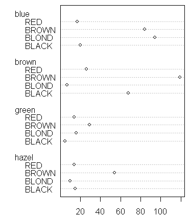
One option for displaying contingency table data is a graphical tool, dotchart:
> dotchart(ct)

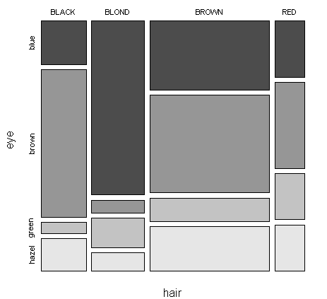
An alternative graphical tool is the mosaic plot, which divides the plot region according to the frequency of each level in a recursive manner:
> mosaicplot(ct,color=T,main="")

In the plot,
the area is first divided according to the frequency of hair color
within each hair color, the area is then divided according to the frequency of eye color
we can easily read the information of pi+ and pj|i from the plot
a different plot could be constructed by reversing the order of hair and eye in the xtabs command above
we can now readily see the frequency of various outcomes. For example, brown hair and brown eyes is the most common combination while black hair and green eyes is the least common
(Q: what patterns will you see in the dotchart and mosaic plots if the two variables are independent? what if they have equivalent marginal proportions? Generate some tables with the two properties and draw the plots.)