We demonstrate the robust methods on the Chicago insurance data. Using least squares on the data:
> chicago <- read.table("chicago.txt")
>
g <- lm(involact ~ race + fire + theft + age + log(income), data
=chicago)
> summary(g)
Call:
lm(formula = involact ~ race + fire + theft + age + log(income),
data = chicago)
Residuals:
Min 1Q Median 3Q Max
-0.85393 -0.16922 -0.03088 0.17890 0.81228
Coefficients:
Estimate Std. Error t value Pr(>|t|)
(Intercept) -3.573976 3.857292 -0.927 0.359582
race 0.009502 0.002490 3.817 0.000449 ***
fire 0.039856 0.008766 4.547 4.76e-05 ***
theft -0.010295 0.002818 -3.653 0.000728 ***
age 0.008336 0.002744 3.038 0.004134 **
log(income) 0.345762 0.400123 0.864 0.392540
---
Signif. codes: 0 '***' 0.001 '**' 0.01 '*' 0.05 '.' 0.1 ' ' 1
Residual standard error: 0.3345 on 41 degrees of freedom
Multiple R-Squared: 0.7517, Adjusted R-squared: 0.7214
F-statistic: 24.83 on 5 and 41 DF, p-value: 2.009e-11
Least squares works well when there are normal errors but can be upset by long-tailed errors. A convenient way to apply the Huber method is to apply the "rlm()" function which is part of the MASS library. The default is to use the Huber method but there are other choices (it's controlled by the "psi" option in function "rlm").
> library(MASS)
> gr <- rlm(involact ~ race + fire + theft + age + log(income), data =chicago)
> summary(gr)
Call: rlm(formula = involact ~ race + fire + theft + age + log(income),
data = chicago)
Residuals:
Min 1Q Median 3Q Max
-0.99015 -0.16183 -0.01694 0.17569 0.89655
Coefficients:
Value Std. Error t value
(Intercept) -2.9257 3.3974 -0.8612
race 0.0079 0.0022 3.5828
fire 0.0459 0.0077 5.9404
theft -0.0097 0.0025 -3.9124
age 0.0064 0.0024 2.6509
log(income) 0.2829 0.3524 0.8029
Residual standard error: 0.2492 on 41 degrees of freedom
Correlation of Coefficients:
(Intercept) race fire theft age
race -0.6537
fire -0.4200 -0.0958
theft 0.2803 -0.1050 -0.5324
age -0.4996 0.2941 0.0098 -0.2366
log(income) -0.9993 0.6501 0.4237 -0.2883 0.4747
The R2 and F-statistics are not given because they cannot be calculated (at least not in the same way). The numerical values of the coefficients have changed a small amount but the general significance of the variables remains the same and our substantive conclusion would not be altered. If you have seen something different, you would need to find out the cause. Perhaps some group of observations were not being fit well and the robust regression excluded these points.
Now try resistant regression methods: least trimmed squares (LTS) and least median of squares (LMS). These methods are the most robust of the methods tried here (in terms of breakdown point):
> library(MASS)
> glts <- ltsreg(involact ~ race + fire + theft + age + log(income), data =chicago)
> glts
Call:
lqs.formula(formula = involact ~ race + fire + theft + age +
log(income), data = chicago, method = "lts")
Coefficients:
(Intercept) race fire theft age log(income)
-2.743009 0.007801 0.046987 -0.008674 0.001060 0.282555
Scale estimates 0.1479 0.1654
> glts <- ltsreg(involact ~ race + fire + theft + age + log(income), data =chicago)
> glts
Call:
lqs.formula(formula = involact ~ race + fire + theft + age +
log(income), data = chicago, method = "lts")
Coefficients:
(Intercept) race fire theft age log(income)
-1.725e+00 5.351e-03 5.138e-02 -8.592e-03 2.706e-05 1.800e-01
Scale estimates 0.1490 0.1818
The default choice of q is [n/2]+[(p+1)/2], where [x] indicates the largest integer less than or equal to x. I repeated the command twice and you will notice that the results are somewhat different. This is because the default genetic algorithm used to compute the coefficients is non-deterministic. An exhaustive search method can be used:
> glts <- ltsreg(involact ~ race + fire + theft + age + log(income), data =chicago, nsamp="exact")
But, it may take a long time to get the result.
> glts
Call:
lqs.formula(formula = involact ~ race + fire + theft + age +
log(income), data = chicago, nsamp = "exact", method = "lts")
Coefficients:
(Intercept) race fire theft age log(income)
-1.1209359 0.0057515 0.0485985 -0.0085099 0.0007616 0.1125155
Scale estimates 0.1342 0.1571
For LMS, you can use:
> glms <- lmsreg(involact ~ race + fire + theft + age + log(income), data =chicago)
> glms
Call:
lqs.formula(formula = involact ~ race + fire + theft + age +
log(income), data = chicago, method = "lms")
Coefficients:
(Intercept) race fire theft age log(income)
-1.9920074 0.0083958 0.0462469 -0.0087194 0.0008802 0.2028362
Scale estimates 0.1254 0.1460
> glms <- lmsreg(involact ~ race + fire + theft + age + log(income), data =chicago)
> glms
Call:
lqs.formula(formula = involact ~ race + fire + theft + age +
log(income), data = chicago, method = "lms")
Coefficients:
(Intercept) race fire theft age log(income)
-5.145357 -0.002059 0.088543 -0.016717 0.005252 0.526124
Scale estimates 0.1509 0.1301
We
have the same problem as in LTS.
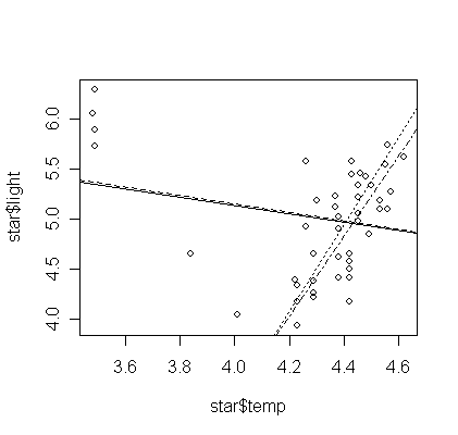
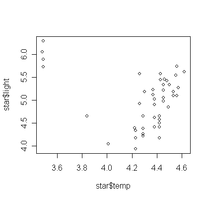
To show why the two methods is more resistant to outliers. Let's take a look of the star data used in outlier test lab:
>
star <- read.table("star.txt",h=T)
>
plot(star$temp,star$light)

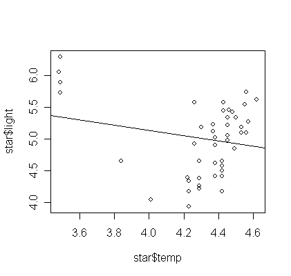
> gs <- lm(light ~ temp, data=star)
>
abline(gs, lty=1)
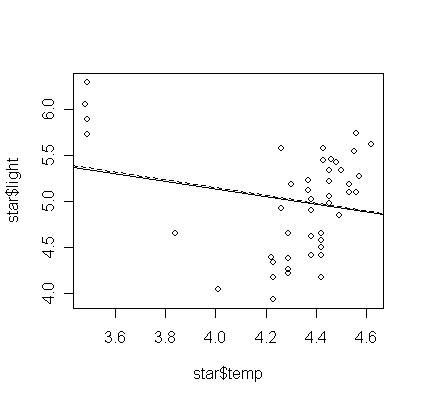
> gsr <- rlm(light ~ temp, data=star)
> abline(gsr, lty=2)
> gslts <- ltsreg(light ~ temp, data=star)
> abline(gslts, lty=3)

> gslms <- lmsreg(light ~ temp, data=star)
> abline(gslms, lty=4)
