Chicago Insurance Redlining (Reading: Faraway (2005, 1st edition), chapter 11)

In a study of insurance availability in Chicago, the U.S. Commission on Civil Rights attempted to examine charges by several community organizations that insurance companies were redlining their neighborhoods, ie. cancelling policies or refusing to insure or renew. First the Illinois Department of Insurance provided the number of cancellations, non-renewals, new policies, and renewals of homeowners and residential fire insurance policies by ZIP code for the months of December 1977 through February 1978. The companies that provided this information account for more than 70% of the homeowners insurance policies written in the City of Chicago. The department also supplied the number of FAIR plan policies written an renewed in Chicago by zip code for the months of December 1977 through May 1978. Since most FAIR plan policyholders secure such coverage only after they have been rejected by the voluntary market, rather than as a result of a preference for that type of insurance, the distribution of FAIR plan policies is another measure of insurance availability in the voluntary market.

Secondly, the Chicago Police Department provided crime data, by beat, on all thefts for the year 1975. Most Insurance companies claim to base their underwriting activities on loss data from the preceding years, i.e. a 2-3 year lag seems reasonable for analysis purposes. the Chicago Fire Department provided similar data on fires occurring during 1975. These fire and theft data were organized by zip code.

Finally the US Bureau of the census supplied data on racial composition, income and age and value of residential units for each ZIP code in Chicago. To adjust for these differences in the populations size associated with different ZIP code areas, the theft data were expressed as incidents per 1,000 population and the fire and insurance data as incidents per 100 housing units.

The variables are

race:          racial composition in percent minority

fire:           fires per 100 housing units

theft:         theft per 1000 population

age:           percent of housing units built before 1939

volact:       new homeowner policies plus renewals minus cancellations and non renewals per 100 housing units

involact:    new FAIR plan policies and renewals per 100 housing units

income:     median family income

The data comes from the book ``Data : a collection of problems from many fields for the student and research worker'' by D. Andrews and A. Herzberg (published by Springer). We choose the Involuntary market activity variable (the number getting FAIR plan insurance) as the response since this seems to be the best measure of those who are denied insurance by others. Note that it is not a perfect measure because some who are denied insurance may give up and others still may not try at all for that reason. 

Furthermore, we do not know the race of those denied insurance. The voluntary market activity variable is not as relevant. We will focus on the relationship between race and the response although similar analyses should be done for the income variable.

Start by reading the data in and examining it:
> chicago <- read.table("chicago.txt")
> chicago

Rescale the income variable and omit volact

> chicago <- data.frame(chicago[,1:4],chicago[,6],chicago[,7]/1000)
> chicago

Fix up the variable names and summarize:

> names(chicago) <- c("race","fire","theft","age","involact","income")
> summary(chicago)

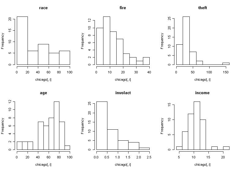
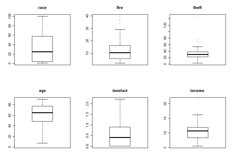
What do you notice? We see that there is a wide range in the race variable with some zip codes being almost entirely minority or non-minority. This is good for our analysis since it will reduce the variation in the regression coefficient for race, allowing us to assess this effect more accurately. If all the zip codes were homogenous, we would never be able to discover an effect from this aggregated data. We also note some skewness in the theft and income variables. The response involact has a large number of zeros. This is not good for the assumptions of the linear model but we have little choice but to proceed.

Now make some graphical summaries:
> par(mfrow=c(2,3))
> for(i in 1:6) hist(chicago[,i],main=names(chicago)[i])

> for(i in 1:6) boxplot(chicago[,i],main=names(chicago)[i])

> pairs(chicago)

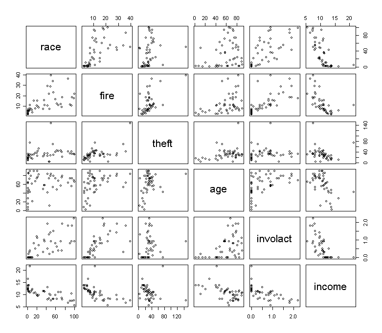
What have you observed from the plots?

Now look at the relationship between involact and race:

> summary(lm(involact ~ race,data=chicago))

We can clearly see that zip codes with high % minority are being denied insurance at higher rate than other zip codes. That is not in doubt. However, can the insurance companies claim that the discrepancy is due to greater risks in some zip-codes? For example, we see that % minority is correlated with the fire rate from the plots. The insurance companies could say that they were denying insurance in neighborhoods where they had sustained large fire-related losses and any discriminatory effect was a by-product of (presumably) legitimate business practice. What can regression analysis tell us about this claim? 

The question of which variables should also be included in the regression so that their effect may be adjusted for is difficult. Statistically, we can do it, but the important question is whether it should be done at all. For example, it's known that the incomes of women is the US are generally lower than those of men. However, if one adjusted for various factors such as type of job and length of service, this gender difference is reduced or can even disappear. The controversy is not statistical but political --- should these factors be used to make the adjustment?

In this example, suppose that if the effect of adjusting for income differences was to remove the race effect? This would pose an interesting but non-statistical question. I have chosen to include the income variable here just to see what happens. I use log(income) partly because of skewness in this variable but also because income is better consider on a multiplicative rather than additive scale. In other word, $1,000 is worth a lot more to a poor person than a millionaire because $1,000 is a much greater fraction of the poor person's wealth.

Now, we start with the full model: 

> g <- lm(involact ~ race + fire + theft + age + log(income), data = chicago)
> summary(g)

Before we start making any conclusions, we should check the model assumptions.

> par(mfrow=c(2,2))

> plot(g)

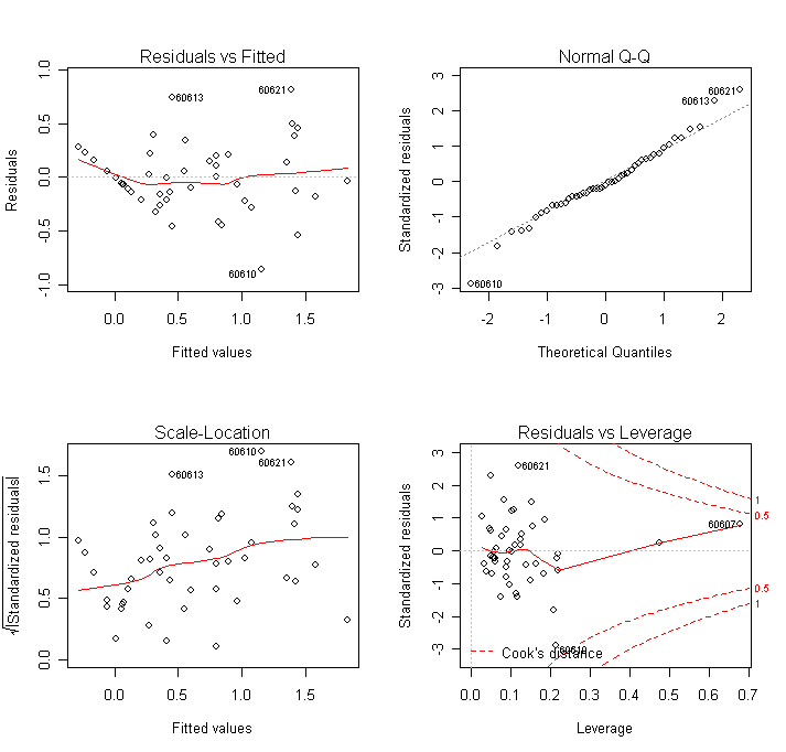
The diagonal streak in the residual-fitted plot is caused by the large number of zero response values in the data. Turning a blind eye to this feature, we see no particular problem. The Q-Q plot looks fine too.

Now, check out the jacknife residuals:

> jack <- rstudent(g)
> qt(0.05/(2*47), 47-6-1)

> jack[ abs(jack) > 3.529468 ]

Nothing too extreme - now look at the Cook statistics. 

> cooks <- cooks.distance(g) 

> row.names(chicago)[cooks>0.1]

Data with zip codes "60610", "60607", "60653", and "60621" correspond to the four largest influence points.

Now let's look at influence - what happens if points are excluded?

> gi <- lm.influence(g)

> par(mfrow=c(2,3))
> for(i in 1:5) {plot(gi$coef[,i+1], main=names(chicago)[-5][i]); abline(h=0); identify(1:47, gi$coef[,i+1], row.names(chicago))}

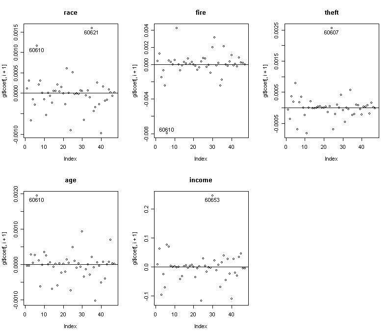
Same points stand up. 

> chicago[c("60610", "60607", "60621", "60653") ,]

Roughly speaking, "60610" and "60607" have high theft and fire, "60621" and "60653" have high race and low income.

See what happens when we exclude these points:

> summary(lm(involact ~ race + fire + theft + age + log(income), subset=(cooks < 0.3), data = chicago))

> summary(lm(involact ~ race + fire + theft + age + log(income), subset=(cooks < 0.2), data = chicago))

> summary(lm(involact ~ race + fire + theft + age + log(income), subset=(cooks < 0.1), data = chicago))

I decide to exclude only the first two zip codes with largest cook's distance, i.e., "60610" and "60607". 

> g <- lm(involact ~ race + fire + theft + age + log(income), subset=(cooks < 0.2), data = chicago)

> summary(g)

After they are excluded, theft and age are no longer significant at the 5% level. We now address the question of transformations - because the response has some zero values and for interpretational reasons we will not try to transform it. Similarly, since the race variable is the primary predictor of interest we won't try transforming it either so as to avoid interpretation difficulties. We try fitting a polynomial model with quadratic terms in each of the predictors:

> g2 <- lm(involact ~ race + poly(fire,2) + poly(theft,2) + poly(age,2) + poly(log(income),2), subset=(cooks <0.2), data = chicago)
> anova(g,g2)

It seems that we can do without the quadratic terms. A check of the partial residual plots also reveals no need to transform. We now move on to variable selection. We are not so much interested in picking one model here because we are mostly interested in the dependency of involact on the race variable. So b_race is the thing we want to focus on. The problem is that collinearity with the other variables may cause b_race to vary substantially depending on what other variables are in the model. We address this question here. leaps() is bit picky about its input format so I need to form the X and Y explicitly:

> y <- chicago$involact[cooks < 0.2]
> x <- cbind(chicago[cooks < 0.2,1:4], linc=log(chicago[cooks < 0.2,6]))
> library(leaps)

> a  <- leaps(x,y)
Now, make the C_p plot:

> par(mfrow=c(1,1))
> plot(a$size, a$Cp, xlab="p", ylab="Cp"); abline(0,1)

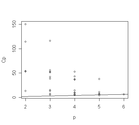
> small <- (a$Cp < 10) 

> plot(a$size[small], a$Cp[small], xlab="p", ylab="Cp"); abline(0,1)

> a.labels <- apply(a$which,1,function(x) paste(as.character((1:5)[x]),collapse="")) 

> text(a$size[small], a$Cp[small], a.labels[small], cex=0.8) 

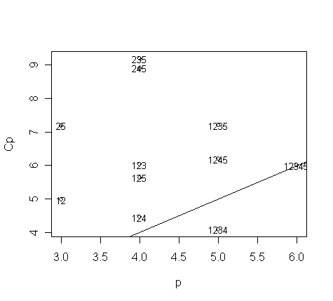
Now, the best model seems to be this one:

> g <- lm(involact ~ race + fire + theft + age, data=chicago, subset=(cooks < 0.2))
> summary(g)

Now fit all the contenders and check out the coefficient for race - you will find it is significant in all of them. The fire rate is also significant and actually has higher t-statistics. Thus, we have verified that there is a positive relationship between involact and race while controlling for a selection of the other variables. This gives us some confidence in asserting that there is a strong relationship that is not sensitive to the choice of predictors.

How robust is the conclusion? Would other analysts have come to the same conclusion? One alternative model is:

> galt <- lm(involact~ race + fire + log(income), data=chicago, subset=(cooks < 0.2))

> summary(galt)

In this model, we see that race is not statistically significant. The previous model did fit slightly better but it is important that there exists a reasonable model in which race is not significant since although the evidence seems fairly strong in favor of a race effect, it is not entirely conclusive. Interestingly enough, if log(income) is dropped:

> galt <- lm(involact~ race + fire, data=chicago, subset=(cooks < 0.2))

> summary(galt)

We find race again becomes significant which raises again the question of whether income should be adjusted for since it makes all the difference here. It's recommended to study the collinearity structure in the predictor to gain more understanding about why it happens.

We now return to the two left-out cases. Observe the difference in the fit when the two are re-included on the best model. The quantities may change but the qualitative message is the same. It is better to include all points if possible, especially in a legal case like this where excluding points might lead to criticism and suspicion of the results.

> g <- lm(involact ~ race + fire + theft + age, data=chicago)
> summary(g)

The main message of the data is not changed - better check the diagnostics:

> par(mfrow=c(2,2)); plot(g)

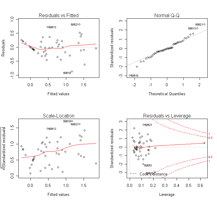
which indicates no trouble. (adding back in the two points to the race+fire+log(income) model made race significant again.) So, it looks like there is some good evidence that zip codes with high minority populations are being "redlined'' - that is improperly denied insurance. While there is evidence that some of the relationship between race and involact can be explained by the fire rate, there is still a component that cannot be attributed to the other variables. However, note that there is some doubt due to the response not being a perfect measure of people being denied insurance - it only appears to be a good substitute. I would guess the effect would be stronger if we did get to see the true response but there is no way to show that with the evidence available. There is also the problem of a potential latent variable that might be the true cause of the observed relationship, but it is difficult to see what that variable might be.

There are some special difficulties in presenting this during a court case. With scientific enquiries, there is always room for uncertainty and subtlety in presenting the results, but this is much more difficult in the court room. The jury may know no statistics and lawyers are clever at twisting words. A statistician giving evidence as an expert witness would do well to keep the message simple.