With real data, you never know the magnitude of the effect of errors in the predictors since we don't observe the true values. In this section we will simulate some data (so we know the true values of the parameters) and then add errors to the predictor to see the effect. First we generate some (xi, yi) pairs and then add increasing amounts of error to x. Remember the error is random so you won't get the exact same results if you repeat this experiment.
> x <- 10*runif(50) # x~U(0,10), 50 uniform random numbers
> y <- x+rnorm(50) # b0=0,
b1=1, e~U(0,1)
> m1 <- lm(y~x) # fit a simple linear regression model
> summary(m1) # should see estimates close to true values
Call:
lm(formula = y ~ x)
Residuals:
Min 1Q Median 3Q Max
-2.39959 -0.64664 0.01070 0.77001 2.20880
Coefficients:
Estimate Std. Error t value Pr(>|t|)
(Intercept) 0.13929 0.28620 0.487 0.629
x 1.00315 0.05738 17.484 <2e-16 ***
---
Signif. codes: 0 '***' 0.001 '**' 0.01 '*' 0.05 '.' 0.1 ' ' 1
Residual standard error: 1.036 on 48 degrees of freedom
Multiple R-Squared: 0.8643, Adjusted R-squared: 0.8615
F-statistic: 305.7 on 1 and 48 DF, p-value: < 2.2e-16
> z <- x+rnorm(50) # now add some standard normal error to x
> m2 <- lm(y~z)
> summary(m2) # what happened to the estimates and the other quantities?
Call:
lm(formula = y ~ z)
Residuals:
Min 1Q Median 3Q Max
-3.68212 -0.84355 0.08807 0.78287 2.70036
Coefficients:
Estimate Std. Error t value Pr(>|t|)
(Intercept) 0.46071 0.34165 1.348 0.184
z 0.91511 0.06687 13.685 <2e-16 ***
---
Signif. codes: 0 '***' 0.001 '**' 0.01 '*' 0.05 '.' 0.1 ' ' 1
Residual standard error: 1.27 on 48 degrees of freedom
Multiple R-Squared: 0.796, Adjusted R-squared: 0.7917
F-statistic: 187.3 on 1 and 48 DF, p-value: < 2.2e-16
> z1 <- x+5*rnorm(50) # add even more error
> m3 <- lm(y~z1)
> summary(m3) # relationship between x and y is almost washed out
Call:
lm(formula = y ~ z1)
Residuals:
Min 1Q Median 3Q Max
-5.34926 -1.54357 -0.01277 1.32366 5.75679
Coefficients:
Estimate Std. Error t value Pr(>|t|)
(Intercept) 3.3447 0.3924 8.524 3.60e-11 ***
z1 0.2443 0.0495 4.935 1.01e-05 ***
---
Signif. codes: 0 '***' 0.001 '**' 0.01 '*' 0.05 '.' 0.1 ' ' 1
Residual standard error: 2.291 on 48 degrees of freedom
Multiple R-Squared: 0.3366, Adjusted R-squared: 0.3228
F-statistic: 24.35 on 1 and 48 DF, p-value: 1.006e-05
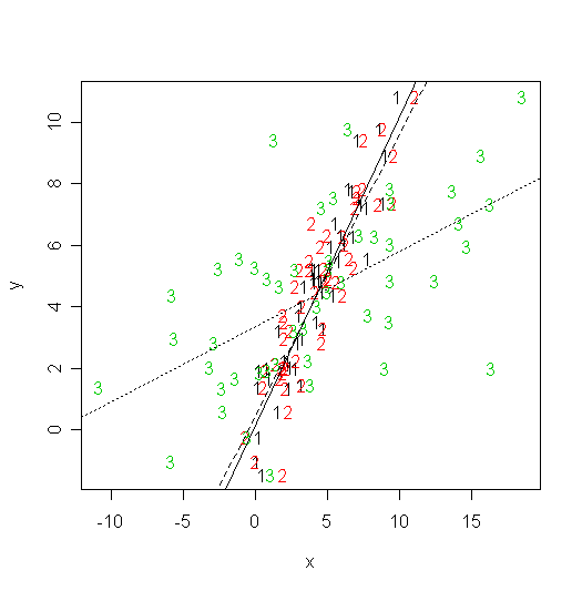
We can plot all this information:
>
matplot(cbind(x,z,z1),y,xlab="x",ylab="y")
> abline(m1,lty=1)
> abline(m2,lty=2)
> abline(m3,lty=3)

Note the slopes decrease when the errors in x have larger variance.
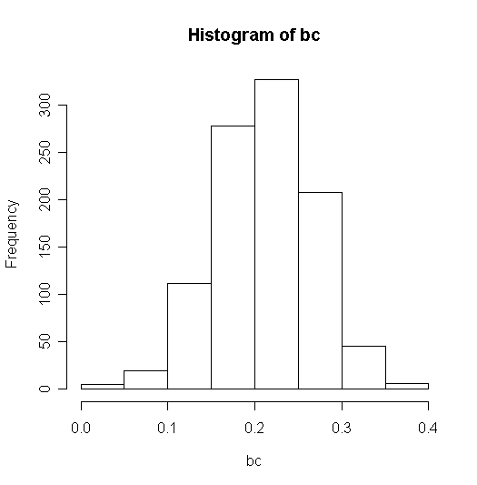
To get an idea of average behavior we need to repeat the experiment (I will do it 1000 times here). The slopes from the 1000 experiments are saved in vector bc:
> bc <- rep(0, 1000)
> for (i in 1:1000) {
+ y <- x + rnorm(50)
+ z <- x + 5*rnorm(50)
+ g <- lm(y~z)
+ bc[i] <- g$coef[2]
+ }
> summary(bc)
Min. 1st Qu. Median Mean 3rd Qu. Max.
0.02461 0.17470 0.21470 0.21220 0.25110 0.38110
> hist(bc)

Given that the variance of a standard uniform random variable is 1/12, sd2=25 and sx2=100/12, we'd expect the mean to be 0.25.