Tesging-based procedure (Reading: Faraway (2005, 1st edition), 8.2)
We illustrate the variable selection methods on a build-in dataset (called "state") in R, which contains some data on the 50 states (use the command "help(state)" to get more information). We will use the data matrix "state.x77" which gives the population estimate as of july 1, 1975; per capita income (1974); illiteracy (1970, percent of population); life expectancy in years (1969-71); murder and non-negligent manslaughter rate per 100,000 population (1976); percent high-school graduates (1970); mean number of days with min temperature < 32 degrees (1931-1960) in capital or large city; and land area in square miles. We will take life expectancy as the response and the remaining variables as predictors - we extract these for convenience and fit the full model.
> data(state)
> statedata <- data.frame(state.x77, row.names=state.abb, check.names=T)
> statedata # take a look
Population Income Illiteracy Life.Exp Murder HS.Grad Frost
Area
AL
3615 3624
2.1 69.05
15.1 41.3
20 50708
AK
365 6315
1.5 69.31
11.3 66.7
152 566432
AZ
2212 4530
1.8 70.55
7.8 58.1 15
113417
… deleted …
WY 376 4566 0.6 70.29 6.9 62.9 173 97203
> g <- lm(Life.Exp ~ ., data=statedata)
> summary(g)
Coefficients:
Estimate Std. Error t value Pr(>|t|)
(Intercept)
7.094e+01 1.748e+00
40.586 < 2e-16 ***
Population
5.180e-05 2.919e-05
1.775 0.0832 .
Income
-2.180e-05 2.444e-04 -0.089
0.9293
Illiteracy
3.382e-02 3.663e-01
0.092 0.9269
Murder
-3.011e-01 4.662e-02 -6.459
8.68e-08 ***
HS.Grad
4.893e-02 2.332e-02 2.098
0.0420 *
Frost
-5.735e-03 3.143e-03 -1.825
0.0752 .
Area
-7.383e-08 1.668e-06 -0.044
0.9649
---
Signif.
codes: 0 `***' 0.001 `**' 0.01 `*'
0.05 `.' 0.1 ` ' 1
Residual
standard error: 0.7448 on 42 degrees of freedom
Multiple
R-Squared: 0.7362, Adjusted
R-squared: 0.6922
F-statistic: 16.74 on 7 and 42 DF, p-value: 2.534e-10
Which predictors should be included - can you tell from the p-values? Looking at the coefficients, can you see what operation would be helpful? Does the murder rate decrease life expectancy - that's obvious a priori but how should these results be interpreted?
We illustrate the backward method --- at each step, we remove the predictor with the largest p-value over 0.05. [Note: In R, the function "mle.stepwise()" in "wle" library can automatically do the job. See the "help(mle.stepwise)" page in R for details.]
> g <- update(g, .~. - Area); summary(g)
Call:
lm(formula = Life.Exp ~ Population + Income + Illiteracy + Murder +
HS.Grad + Frost, data = statedata)
Residuals:
Min 1Q Median 3Q Max
-1.49047 -0.52533 -0.02546 0.57160 1.50374
Coefficients:
Estimate Std. Error t value Pr(>|t|)
(Intercept) 7.099e+01 1.387e+00 51.165 < 2e-16 ***
Population 5.188e-05 2.879e-05 1.802 0.0785 .
Income -2.444e-05 2.343e-04 -0.104 0.9174
Illiteracy 2.846e-02 3.416e-01 0.083 0.9340
Murder -3.018e-01 4.334e-02 -6.963 1.45e-08 ***
HS.Grad 4.847e-02 2.067e-02 2.345 0.0237 *
Frost -5.776e-03 2.970e-03 -1.945 0.0584 .
---
Signif. codes: 0 '***' 0.001 '**' 0.01 '*' 0.05 '.' 0.1 ' ' 1
Residual standard error: 0.7361 on 43 degrees of freedom
Multiple R-Squared: 0.7361, Adjusted R-squared: 0.6993
F-statistic: 19.99 on 6 and 43 DF, p-value: 5.362e-11
> g <- update(g, .~. - Illiteracy); summary(g)
Call:
lm(formula = Life.Exp ~ Population + Income + Murder + HS.Grad +
Frost, data = statedata)
Residuals:
Min 1Q Median 3Q Max
-1.48921 -0.51224 -0.03290 0.56447 1.51662
Coefficients:
Estimate Std. Error t value Pr(>|t|)
(Intercept) 7.107e+01 1.029e+00 69.067 < 2e-16 ***
Population 5.115e-05 2.709e-05 1.888 0.0657 .
Income -2.477e-05 2.316e-04 -0.107 0.9153
Murder -3.000e-01 3.704e-02 -8.099 2.91e-10 ***
HS.Grad 4.776e-02 1.859e-02 2.569 0.0137 *
Frost -5.910e-03 2.468e-03 -2.395 0.0210 *
---
Signif. codes: 0 '***' 0.001 '**' 0.01 '*' 0.05 '.' 0.1 ' ' 1
Residual standard error: 0.7277 on 44 degrees of freedom
Multiple R-Squared: 0.7361, Adjusted R-squared: 0.7061
F-statistic: 24.55 on 5 and 44 DF, p-value: 1.019e-11
> g <- update(g, .~. - Income); summary(g)
Call:
lm(formula = Life.Exp ~ Population + Murder + HS.Grad + Frost,
data = statedata)
Residuals:
Min 1Q Median 3Q Max
-1.47095 -0.53464 -0.03701 0.57621 1.50683
Coefficients:
Estimate Std. Error t value Pr(>|t|)
(Intercept) 7.103e+01 9.529e-01 74.542 < 2e-16 ***
Population 5.014e-05 2.512e-05 1.996 0.05201 .
Murder -3.001e-01 3.661e-02 -8.199 1.77e-10 ***
HS.Grad 4.658e-02 1.483e-02 3.142 0.00297 **
Frost -5.943e-03 2.421e-03 -2.455 0.01802 *
---
Signif. codes: 0 '***' 0.001 '**' 0.01 '*' 0.05 '.' 0.1 ' ' 1
Residual standard error: 0.7197 on 45 degrees of freedom
Multiple R-Squared: 0.736, Adjusted R-squared: 0.7126
F-statistic: 31.37 on 4 and 45 DF, p-value: 1.696e-12
> g <- update(g, .~. - Population); summary(g)
Call:
lm(formula = Life.Exp ~ Murder + HS.Grad + Frost, data = statedata)
Residuals:
Min 1Q Median 3Q Max
-1.5015 -0.5391 0.1014 0.5921 1.2268
Coefficients:
Estimate Std. Error t value Pr(>|t|)
(Intercept) 71.036379 0.983262 72.246 < 2e-16 ***
Murder -0.283065 0.036731 -7.706 8.04e-10 ***
HS.Grad 0.049949 0.015201 3.286 0.00195 **
Frost -0.006912 0.002447 -2.824 0.00699 **
---
Signif. codes: 0 '***' 0.001 '**' 0.01 '*' 0.05 '.' 0.1 ' ' 1
Residual standard error: 0.7427 on 46 degrees of freedom
Multiple R-Squared: 0.7127, Adjusted R-squared: 0.6939
F-statistic: 38.03 on 3 and 46 DF, p-value: 1.634e-12
The final removal of the Population variable is a close call. We may want to consider including this variable if interpretation is aided. Notice that the R2 for the full model of 0.736 is reduced only slightly to 0.713 in the final model. Thus the removal of four predictors causes only a minor reduction in fit (Note the adjusted R2 increases).
It is important to understand that the variables omitted from the model may still be related to the response. For example, let us fit a model with Illiteracy, Murder, and Frost as predictors:
> summary(lm(Life.Exp~Illiteracy+Murder+Frost, statedata))
Call:
lm(formula = Life.Exp ~ Illiteracy + Murder + Frost, data = statedata)
Residuals:
Min 1Q Median 3Q Max
-1.590098 -0.469608 0.003935 0.570604 1.922922
Coefficients:
Estimate Std. Error t value Pr(>|t|)
(Intercept) 74.556717 0.584251 127.611 < 2e-16 ***
Illiteracy -0.601761 0.298927 -2.013 0.04998 *
Murder -0.280047 0.043394 -6.454 6.03e-08 ***
Frost -0.008691 0.002959 -2.937 0.00517 **
---
Signif. codes: 0 '***' 0.001 '**' 0.01 '*' 0.05 '.' 0.1 ' ' 1
Residual standard error: 0.7911 on 46 degrees of freedom
Multiple R-Squared: 0.6739, Adjusted R-squared: 0.6527
F-statistic: 31.69 on 3 and 46 DF, p-value: 2.915e-11
We can see that Illiteracy does have some association with Life Expectancy although Illiteracy was removed during the backward selection. It is true that replacing Illiteracy with High School graduation rate gave us a somewhat better fitted model in terms of R2. But, it would be insufficient to conclude that Illiteracy is not a variable of interest. This example also shows one drawback of testing-based procedure: when there are several models that can fit the data equally well, the testing-based procedure ends up with only one model and offers no information about other good fitted models.
Criterion-based procedure (Reading: Faraway (2005, 1st edition), 8.3)
Now, let's try some criterion-based methods. Let's start from the AIC. In R, AIC for model selection is implemented with a stepwise procedure in the function "step()" or "stepAIC()". The function does not evaluate the AIC for all possible models but uses a search method ("forward", "backward", or "both", default is "both") that compares models sequentially. Thus it bears some comparison to the stepwise method described above but with the advantage that no dubious p-values are used.
> g <- lm(Life.Exp ~ ., data=statedata)
> step(g)
Start:
AIC= -22.18
Life.Exp
~ Population + Income + Illiteracy + Murder + HS.Grad +
Frost + Area
Df Sum of Sq RSS
AIC
-
Area 1 0.001
23.298 -24.182
-
Income 1 0.004
23.302 -24.175
-
Illiteracy 1 0.005
23.302 -24.174
<none>
23.297 -22.185
-
Population 1 1.747
25.044 -20.569
-
Frost 1 1.847
25.144 -20.371
-
HS.Grad 1 2.441
25.738 -19.202
-
Murder 1 23.141 46.438
10.305
Step:
AIC= -24.18
Life.Exp
~ Population + Income + Illiteracy + Murder + HS.Grad +
Frost
Df Sum of Sq RSS
AIC
-
Illiteracy 1 0.004
23.302 -26.174
-
Income 1 0.006
23.304 -26.170
<none>
23.298 -24.182
-
Population 1 1.760
25.058 -22.541
-
Frost 1 2.049
25.347 -21.968
-
HS.Grad 1 2.980
26.279 -20.163
-
Murder 1 26.272 49.570
11.568
Step:
AIC= -26.17
Life.Exp
~ Population + Income + Murder + HS.Grad + Frost
Df Sum of Sq RSS
AIC
-
Income 1 0.006
23.308 -28.161
<none>
23.302 -26.174
-
Population 1 1.887
25.189 -24.280
-
Frost 1 3.037
26.339 -22.048
-
HS.Grad 1 3.495
26.797 -21.187
-
Murder 1 34.739 58.041
17.457
Step:
AIC= -28.16
Life.Exp
~ Population + Murder + HS.Grad + Frost
Df Sum of Sq RSS
AIC
<none>
23.308 -28.161
-
Population 1 2.064
25.372 -25.920
-
Frost 1 3.122
26.430 -23.876
-
HS.Grad 1 5.112
28.420 -20.246
-
Murder 1 34.816 58.124
15.528
Call:
lm(formula
= Life.Exp ~ Population + Murder + HS.Grad + Frost, data = statedata)
Coefficients:
(Intercept)
Population Murder
HS.Grad
Frost
7.103e+01 5.014e-05 -3.001e-01 4.658e-02 -5.943e-03
The sequence of variable removal is the same as with backward elimination. The only difference is the Population variable is retained.
Now we try the Cp and adjusted R2 methods for the selection of variables in the State dataset. The function "leaps()" supports the Mallow's Cp and adjusted R2 criteria. The default for the function is the Mallow's Cp criterion:
> library(leaps)
>
x <- statedata[,-4]
> y <- statedata[,4]
> gcp <-
leaps(x,y)
> gcp
$which
1 2 3 4 5 6 7
1 FALSE FALSE FALSE TRUE FALSE FALSE FALSE
1 FALSE FALSE TRUE FALSE FALSE FALSE FALSE
1 FALSE FALSE FALSE FALSE TRUE FALSE FALSE
1 FALSE TRUE FALSE FALSE FALSE FALSE FALSE
1 FALSE FALSE FALSE FALSE
FALSE TRUE FALSE
1 FALSE FALSE FALSE FALSE FALSE
FALSE TRUE
1 TRUE FALSE FALSE FALSE FALSE FALSE
FALSE
2 FALSE FALSE FALSE TRUE TRUE FALSE FALSE
2 TRUE FALSE FALSE TRUE FALSE FALSE FALSE
2 FALSE FALSE FALSE TRUE FALSE TRUE FALSE
2 FALSE TRUE FALSE TRUE FALSE FALSE FALSE
2 FALSE FALSE FALSE TRUE FALSE FALSE TRUE
2 FALSE FALSE TRUE TRUE FALSE FALSE FALSE
2 FALSE FALSE FALSE FALSE TRUE FALSE TRUE
2 FALSE FALSE TRUE FALSE TRUE FALSE FALSE
2 FALSE FALSE TRUE FALSE FALSE TRUE FALSE
2 FALSE TRUE TRUE FALSE FALSE FALSE FALSE
3 FALSE FALSE FALSE TRUE TRUE TRUE FALSE
3 TRUE FALSE FALSE TRUE TRUE FALSE FALSE
3 FALSE TRUE FALSE TRUE FALSE TRUE FALSE
3 TRUE FALSE FALSE TRUE FALSE TRUE FALSE
3 FALSE FALSE TRUE TRUE FALSE TRUE FALSE
3 FALSE FALSE TRUE TRUE TRUE FALSE FALSE
3 FALSE FALSE FALSE TRUE TRUE FALSE TRUE
3 TRUE TRUE FALSE TRUE FALSE FALSE FALSE
3 FALSE TRUE FALSE TRUE TRUE FALSE FALSE
3 TRUE FALSE FALSE TRUE FALSE FALSE TRUE
4 TRUE FALSE FALSE TRUE TRUE TRUE FALSE
4 FALSE TRUE FALSE TRUE TRUE TRUE FALSE
4 FALSE FALSE TRUE TRUE TRUE TRUE FALSE
4 FALSE FALSE FALSE TRUE TRUE TRUE TRUE
4 TRUE FALSE TRUE TRUE TRUE FALSE FALSE
4 TRUE FALSE FALSE TRUE TRUE FALSE TRUE
4 TRUE TRUE FALSE TRUE TRUE FALSE FALSE
4 TRUE TRUE FALSE TRUE FALSE TRUE FALSE
4 TRUE FALSE FALSE TRUE FALSE TRUE TRUE
4 FALSE TRUE TRUE TRUE FALSE TRUE FALSE
5 TRUE TRUE FALSE TRUE TRUE TRUE FALSE
5 TRUE FALSE TRUE TRUE TRUE TRUE FALSE
5 TRUE FALSE FALSE TRUE TRUE TRUE TRUE
5 FALSE TRUE TRUE TRUE TRUE TRUE FALSE
5 FALSE TRUE FALSE TRUE TRUE TRUE TRUE
5 TRUE FALSE TRUE TRUE TRUE FALSE TRUE
5 FALSE FALSE TRUE TRUE TRUE TRUE TRUE
5 TRUE TRUE TRUE TRUE TRUE FALSE FALSE
5 TRUE FALSE TRUE TRUE FALSE TRUE TRUE
5 TRUE TRUE TRUE TRUE FALSE TRUE FALSE
6 TRUE TRUE TRUE TRUE TRUE TRUE FALSE
6 TRUE FALSE TRUE TRUE TRUE TRUE TRUE
6 TRUE TRUE FALSE TRUE TRUE TRUE TRUE
6 FALSE TRUE TRUE TRUE TRUE TRUE TRUE
6 TRUE TRUE TRUE TRUE TRUE FALSE TRUE
6 TRUE TRUE TRUE TRUE FALSE TRUE TRUE
6 TRUE TRUE TRUE FALSE TRUE TRUE TRUE
7 TRUE TRUE TRUE TRUE TRUE TRUE TRUE
$label
[1] "(Intercept)" "1"
"2"
"3"
"4"
[6] "5"
"6"
"7"
$size
[1] 2 2 2 2 2 2 2 3 3 3 3 3 3 3 3 3 3 4 4
4 4 4 4 4 4 4 4 5 5 5 5 5 5 5 5 5 5 6 6 6
[41] 6 6 6 6 6 6 6 7 7 7 7 7 7
7 8
$Cp
[1]
16.126760 58.058325 59.225241 94.755684 102.252357 111.351299
112.447938
[8] 9.669894 10.886508 12.475673 13.791499 17.280014 17.634184 44.940876
[15] 49.351549 54.896851 58.701223 3.739878 5.647595 8.727618 9.236254
[22] 9.903176 10.873258 11.169557 11.190554 11.485646 11.705240 2.019659
[29] 5.411184 5.430093 5.693495 5.780351 7.482910 7.484304 8.309352
[36] 8.884194 9.015565 4.008737 4.012588 4.018235 7.174687 7.306932
[43] 7.344256 7.428952 7.695471 8.888310 9.375028 6.001959 6.007958
You may observe that not all sub-models are reported (only 55 models in this case). The number of reported best models is controlled by the option "nbest" in "leaps" function.
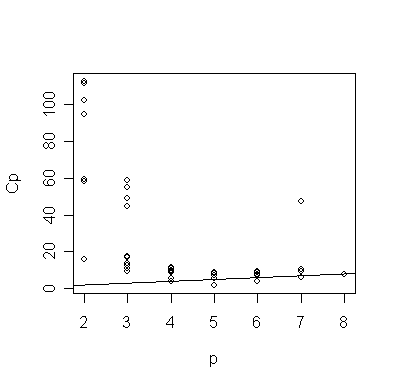
It's usual to plot the Cp data against p:
> plot(gcp$size, gcp$Cp, xlab="p", ylab="Cp"); abline(0,1)

The plot is distorted by the large Cp values - let's exclude them:
> small <- (gcp$Cp < 20) # logical vector of Cp values smaller than 20
> plot(gcp$size[small], gcp$Cp[small], xlab="p", ylab="Cp"); abline(0,1) # plot Cp against p for Cp < 20
> gcp.labels <- apply(gcp$which,1,function(x) paste(as.character((1:7)[x]),collapse="")) # generate model labels
> text(gcp$size[small], gcp$Cp[small], gcp.labels[small]) # add the model labels
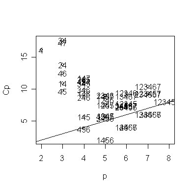
The models are denoted by indices for the predictors. The competition is between the "456" model, i.e., the Forest, HS graduation, and Murder model, and the model also including Population. Both models are on or below the Cp=p line, indicating good fits. The choice is between the smaller model and the larger model which fits a little better. Some even larger models fit in the sense that they are on or below the Cp=p line but we would not opt for these in the presence of smaller models that fit.
Now let's see which model the adjusted R2 criterion selects.
> gadjr <- leaps(x, y, method="adjr2")
> gadjr # take a look
Let's look at the 10 best (in the sense of having high adjusted R2):
> gadjr.labels <- apply(gadjr$which,1,function(x) paste(as.character((1:7)[x]),collapse=""))
> names(gadjr$adjr2) <- gadjr.labels
>
i <- order(gadjr$adjr2, decreasing = T)
> round(gadjr$adjr2[i[1:10]],
3)
1456 12456 13456 14567 123456 134567 124567 456 1234567 2456
0.713 0.706 0.706 0.706 0.699 0.699 0.699 0.694 0.692 0.689
How does this compare to previous results? We can see that the model with Population, Frost, HS graduation, and Murder model has the largest adjusted R2. The best three predictor model picked by Cp is in 8th place but the intervening models are not attractive since they use more predictors than the best model.
Variable selection methods are sensitive to outliers and influential points. Let's check for high leverage points:
>
h <- hat(x)
> names(h) <- state.abb
> rev(sort(h))[1:8]
AK
CA
HI
NV
NM
TX
NY WA
0.8095223 0.4088569 0.3787617 0.3652458 0.3247216 0.2841635 0.2569498 0.2226820
Which state sticks out? Let's try excluding it (Alaska is the second state in the data):
> l <- leaps(x[-2,],y[-2],method="adjr2")
> l.labels <- apply(l$which,1,function(x) paste(as.character((1:7)[x]),collapse=""))
> names(l$adjr2) <- l.labels
>
i <- order(l$adjr2, decreasing = T)
> round(l$adjr2[i[1:10]], 3)
14567 1456 124567 24567 134567 13456 12456 1234567 234567 4567
0.710 0.709 0.707 0.707 0.704 0.703 0.703 0.701 0.700 0.700
Compare with the "best" model selected above. We see that Area now makes it into the model.
Transforming the predictors can also have an effect. Let's take a look at the variables:
> par(mfrow=c(3,3))
>
for (i in c(1:3, 5:8)) boxplot(state.x77[,i],
main=dimnames(state.x77)[[2]][i])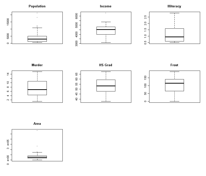
We see that Population, Illiteracy and Area are skewed - we try transforming them:
> nx <- cbind(log(x[,1]),x[,2],log(x[,3]),x[,4:6],log(x[,7]))
And now replot:
> par(mfrow=c(3,3))
> apply(nx,2,boxplot)
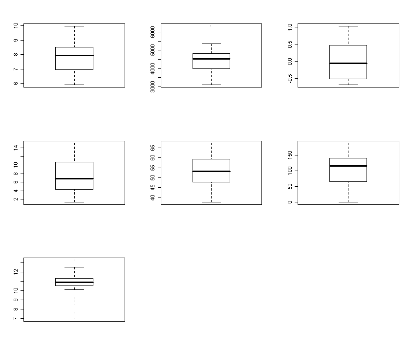
It shows the appropriately transformed data.
Now try the adjusted R2 method again - we make sure the columns of the new matrix have the right label names for ease of reference.
>
dimnames(nx)[[2]] <-
c("logpop","income","logillit","murder","grad","frost","logarea")
> a
<- leaps(nx,y,method="adjr2")
> a.labels <- apply(a$which,1,function(x) paste(as.character((1:7)[x]),collapse=""))
> names(a$adjr2) <- a.labels
>
i <- order(a$adjr2, decreasing = T)
> round(a$adjr2[i[1:10]], 3)
1456 14567 13456 12456 134567 124567 123456 1345 1234567 13457
0.717 0.714 0.712 0.711 0.708 0.707 0.705 0.703 0.701 0.699
This changes the "best" model yet again to log(Population), Frost, HS graduation, and Murder. Compare the maximum adjusted R2 for all the "best" models we have seen Which model will you choose?