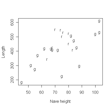
The data for this example consist of
x= nave height and
y = total length in feet for English medieval cathedrals.
Some are in the Romanesque (r) style and others are in the Gothic (g) style. Some cathedrals have parts in both styles and are listed twice.
We wish to investigate how the length is related to height for the two styles. Read in the data and make a summary on the two styles separately.
>
cathedral <- read.table("cathedral.data")
> cathedral # take a
look
style x y
Durham r 75 502
Canterbury r 80 522
...deleted...
Old.St.Paul g 103 611
Salisbury g 84 473
> lapply(split(cathedral, cathedral$style),summary) # "split" divides the data into groups; "lapply" applies a function (in the case, the "summary") over a list of data (in the case, the two groups of data defined by style)
$g
style x y
g:16 Min. : 45.00 Min. :182.0
r: 0 1st Qu.: 60.75 1st Qu.:298.8
Median : 73.50 Median :412.0
Mean : 74.94 Mean :397.4
3rd Qu.: 86.50 3rd Qu.:481.3
Max. :103.00 Max. :611.0
$r
style x y
g:0 Min. :64.00 Min. :344.0
r:9 1st Qu.:70.00 1st Qu.:425.0
Median :75.00 Median :502.0
Mean :74.44 Mean :475.4
3rd Qu.:80.00 3rd Qu.:530.0
Max. :83.00 Max. :551.0
Notice that in this case the two groups have about the same average heights.
Look at the difference in the lengths.
Now plot the data:
>
plot(cathedral$x,cathedral$y,type="n",xlab="Nave height",ylab="Length")
>
text(cathedral$x,cathedral$y,as.character(cathedral$s))
Q: What information have you gathered from the summary and the plot?
Before fitting model, examine how R treat the data:
> is.factor(cathedral$style); is.numeric(cathedral$x); is.numeric(cathedral$y)
style is treated as a qualitative variable and x and y as quantitative variables.
Let's start from fitting the full model, i.e., separate regression lines for each groups.
>
g <- lm(y ~ x+style+x:style, data=cathedral) # to understand the meaning of
"x:style", check "help(formula)". Notice that the model can be equivalently
written as "y~x*style" in R.
> summary(g)
Coefficients:
Estimate Std. Error t value Pr(>|t|)
(Intercept) 37.111 85.675 0.433 0.669317
x
4.808
1.112 4.322 0.000301
***
styler
204.722
347.207 0.590
0.561733
x:styler -1.669 4.641 -0.360 0.722657
---
Signif. codes: 0 `***' 0.001 `**' 0.01 `*' 0.05 `.' 0.1
` ' 1
Residual standard error: 79.11
on 21 degrees of freedom
Multiple R-Squared:
0.5412, Adjusted
R-squared: 0.4757
F-statistic: 8.257 on 3 and 21 DF, p-value: 0.0008072
Q: Do you know how to interpret the estimated parameters in the output?
You must first understand what coding you are using.
Because style is non-numeric, R automatically treats it as a qualitative variables and sets up a coding - but which coding?
> model.matrix(g)
(Intercept)
x
styler x:styler
Durham
1 75 1 75
Canterbury
1 80 1 80
Gloucester
1 68 1 68
Hereford
1 64 1 64
Norwich
1 83 1 83
Peterborough
1 80 1 80
St.Albans
1 70 1 70
Winchester
1 76 1 76
Ely
1 74 1 74
York
1 100
0
0
Bath 1 75 0
0
Bristol
1 52 0
0
Chichester
1 62 0
0
Exeter
1 68 0
0
GloucesterG
1 86 0
0
Lichfield
1 57 0
0
Lincoln
1 82 0
0
NorwichG
1 72 0
0
Ripon
1 88 0
0
Southwark
1 55 0
0
Wells
1 67 0
0
St.Asaph
1 45 0
0
WinchesterG
1 103
0
0
Old.St.Paul
1 103
0
0
Salisbury
1 84 0
0
attr(,"assign")
[1] 0 1 2 3
attr(,"contrasts")
attr(,"contrasts")$style
[1] "contr.treatment"
The Romanesque (r) style is coded as 1 and the Gothic (g) style is coded as 0.
That is, Gothic style is treated as the reference.
This coding is assigned by the contrast function "contr.treatment" in R.
Suppose you would like to code the two groups as 1 and -1, individually. You can use the contrast function "contr.sum" and the following command:
> options(contrasts=c("contr.sum","contr.poly")) # use "help(options)" to understand how to assign contrast
Let's fit the full model again under (-1, 1) coding:
>
g <- lm(y ~ x+style+x:style, data=cathedral)
> summary(g)
Coefficients:
Estimate Std. Error t value Pr(>|t|)
(Intercept) 139.4718 173.6037 0.803 0.431
x
3.9728
2.3206 1.712 0.102
style1 -102.3610 173.6037 -0.590 0.562
x:style1 0.8347 2.3206 0.360 0.723
Residual standard error: 79.11
on 21 degrees of freedom
Multiple R-Squared:
0.5412, Adjusted
R-squared: 0.4757
F-statistic: 8.257 on 3 and 21 DF, p-value: 0.0008072
Compare to the result under (0, 1) coding.
What's different and what's the same? Can you explain why?
Let's take a look of the model matrix under (-1, 1) coding:
> model.matrix(g)
(Intercept) x style1
x:style1
Durham
1 75 -1 -75
Canterbury
1 80 -1 -80
Gloucester
1 68 -1 -68
Hereford
1 64 -1 -64
Norwich
1 83 -1 -83
Peterborough
1 80 -1 -80
St.Albans
1 70 -1 -70
Winchester
1 76 -1 -76
Ely
1 74 -1 -74
York
1 100 1 100
Bath
1 75 1 75
Bristol
1 52 1 52
Chichester
1 62 1 62
Exeter
1 68 1 68
GloucesterG
1 86 1 86
Lichfield
1 57 1 57
Lincoln
1 82 1 82
NorwichG
1 72 1 72
Ripon
1 88 1 88
Southwark
1 55 1 55
Wells
1 67 1 67
St.Asaph
1 45 1 45
WinchesterG
1 103
1
103
Old.St.Paul
1 103
1
103
Salisbury
1 84 1 84
attr(,"assign")
[1] 0 1 2 3
attr(,"contrasts")
attr(,"contrasts")$style
[1] "contr.sum"
Now, let's go back to (0, 1) coding:
> options(contrasts=c("contr.treatment","contr.poly"))
We see that the full model under (0, 1) coding can be simplified to:
>
g1 <- lm(y ~ x+style, data=cathedral)
> summary(g1)
Coefficients:
Estimate Std. Error t value Pr(>|t|)
(Intercept) 44.298 81.648 0.543 0.5929
x
4.712
1.058 4.452 0.0002 ***
styler
80.393
32.306 2.488 0.0209 *
---
Signif. codes: 0 `***' 0.001 `**' 0.01 `*' 0.05 `.' 0.1
` ' 1
Residual standard error: 77.53
on 22 degrees of freedom
Multiple R-Squared:
0.5384, Adjusted
R-squared: 0.4964
F-statistic: 12.83 on 2 and 22 DF, p-value: 0.0002028
Put the two parallel regression on the plot:
>
abline(44.298,4.7116)
> abline(44.298+80.393,4.7116,lty=2)
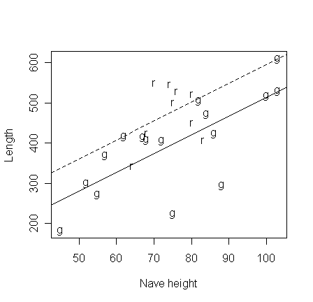
Check out the diagnostics:
>
par(mfrow=c(2,2))
> plot(g)
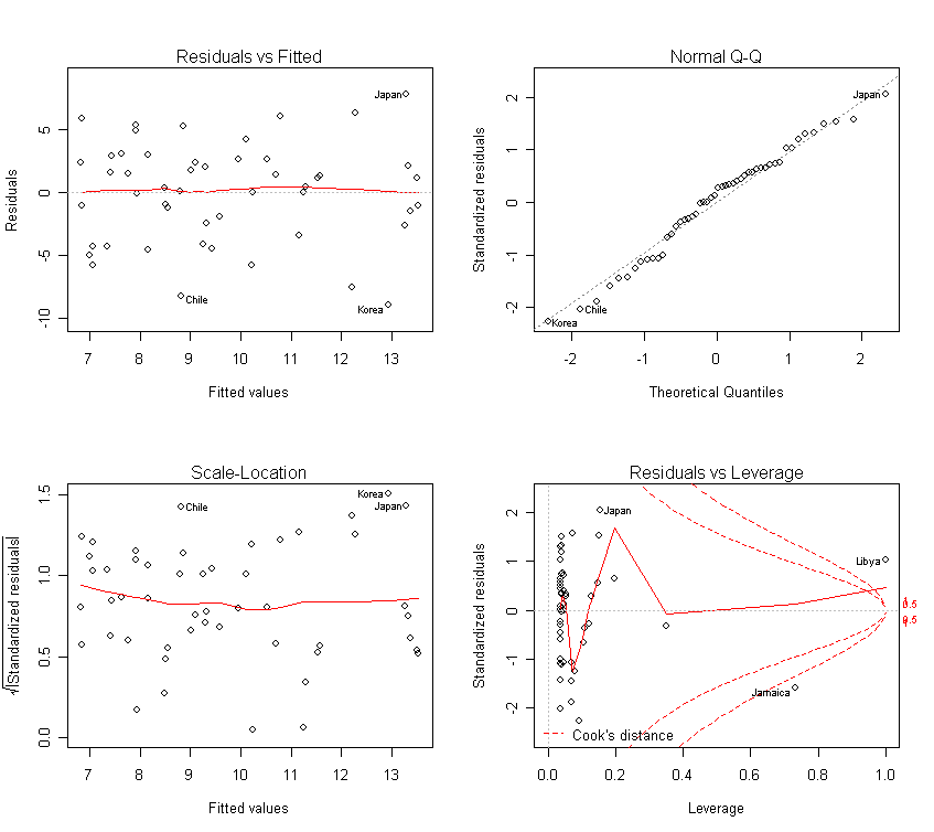
The check on the diagnostics reveals no particular problems.
Our conclusion is that for cathedrals of the same height, Romanesque ones are about 80 (=2*40.2) feet longer.
For each extra foot height, both types of cathedral are about 4.7 feet longer.
Suppose you want to perform an analysis of covariance. You can do it as follows:
>
g2 <- lm(y~x, cathedral)
> anova(g1, g2)
Analysis of Variance Table
Model 1: y ~ x + style
Model 2: y ~ x
Res.Df RSS Df Sum of Sq F Pr(>F)
1 22 132223
2 23 169440 -1 -37217 6.1924 0.02089 *
---
Signif. codes: 0 '***' 0.001 '**' 0.01 '*' 0.05 '.' 0.1 ' ' 1
But, of course, you know it will be the same as the t-test for style in model g1.
Polytomous predictor (Reading: Faraway (2005), 13.2, 13.3)
The data for this example come from a 1966 paper by Cyril Burt entitled "The genetic determination of differences in intelligence: A study of monozygotic twins reared apart".
The data consist of IQ scores for identical twins, one raised by foster parents, the other by the natural parents.
We also know the social class of natural parents (high, middle or low).
We are interested in predicting the IQ of the twin with foster parents from the IQ of the twin with the natural parents and the social class of natural parents.
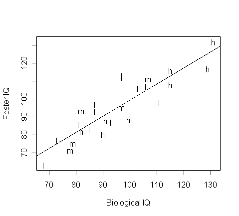
Let's read in and take a look at the data:
>
twins <- read.table("twin.data",header=T)
> twins
Foster Biological Social
1 82 82 high
...deleted...
7 132 131 high
8 71 78 middle
...deleted...
13 111 107 middle
14 63 68 low
...deleted...
27 98 111 low
>
plot(twins$B,twins$F,type="n",xlab="Biological IQ",ylab="Foster IQ")
>
text(twins$B,twins$F,substring(as.character(twins$S),1,1))
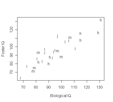
From the plot, what model seems appropriate?
The most general model we'll consider is to fit separate lines for each groups:
>
g <- lm(Foster ~ Biological*Social, twins)
> summary(g)
Coefficients:
Estimate
Std. Error t value Pr(>|t|)
(Intercept)
-1.872044 17.808264 -0.105 0.917
Biological
0.977562 0.163192 5.990 6.04e-06 ***
Sociallow
9.076654 24.448704 0.371 0.714
Socialmiddle
2.688068 31.604178 0.085 0.933
Biological:Sociallow -0.029140 0.244580 -0.119 0.906
Biological:Socialmiddle
-0.004995 0.329525 -0.015 0.988
---
Signif. codes: 0 `***' 0.001 `**' 0.01 `*' 0.05 `.' 0.1
` ' 1
Residual standard error: 7.921
on 21 degrees of freedom
Multiple R-Squared:
0.8041, Adjusted
R-squared: 0.7574
F-statistic: 17.24 on 5 and 21 DF, p-value: 8.31e-07
Q: What do those coefficients mean?
Must know the coding to determine this:
> model.matrix(g)
(Intercept) Biological Sociallow
Socialmiddle Biological:Sociallow Biological:Socialmiddle
1
1
82
0
0
0
0
2
1
90
0
0
0
0
3
1
91
0
0
0
0
4
1
115
0
0
0
0
5
1
115
0
0
0
0
6
1
129
0
0
0
0
7
1
131
0
0
0
0
8
1
78
0
1
0
78
9
1
79
0
1
0
79
10
1
82
0
1
0
82
11
1
97
0
1
0
97
12
1
100
0
1
0
100
13
1
107
0
1
0
107
14
1
68
1
0
68
0
15
1
73
1
0
73
0
16
1
81
1
0
81
0
17
1
85
1
0
85
0
18
1
87
1
0
87
0
19
1
87
1
0
87
0
20
1
93
1
0
93
0
21
1
94
1
0
94
0
22
1
95
1
0
95
0
23
1
97
1
0
97
0
24
1
97
1
0
97
0
25
1
103
1
0
103
0
26
1
106
1
0
106
0
27 1
111
1
0
111
0
attr(,"assign")
[1] 0 1 2 2 3
3
attr(,"contrasts")
attr(,"contrasts")$Social
[1] "contr.treatment"
We can see that the reference is "high" class, being first alphabetically.
The intercept and slope for "low" class line would be (-1.872044 + 9.076654) and (0.977562 -0.029140)
the intercept and slope for "middle" class line would be (-1.872044 + 2.688068) and (0.977562 -0.004995).
Now see if the model can be simplified to the parallel lines model:
>
gp<- lm(Foster ~ Biological+Social, twins)
> anova(gp,g)
Analysis of Variance Table
Model 1: Foster ~ Biological +
Social
Model 2: Foster ~ Biological +
Social + Biological:Social
Res.Df RSS Df Sum of Sq F Pr(>F)
1 23 1318.40
2 21 1317.47 2 0.93 0.0074 0.9926
Yes it can.
The sequential testing can be done in one go:
> anova(g)
Analysis of Variance Table
Response: Foster
Df Sum Sq Mean Sq F value
Pr(>F)
Biological
1 5231.1 5231.1 83.3823
9.28e-09 ***
Social
2 175.1 87.6 1.3958 0.2697
Biological:Social 2 0.9 0.5 0.0074 0.9926
Residuals
21 1317.5
62.7
---
Signif. codes: 0 `***' 0.001 `**' 0.01 `*' 0.05 `.' 0.1 ` ' 1
We see that a further reduction to a single line model is possible:
> gs <- lm(Foster ~ Biological, twins)
> anova(gs,gp)
Analysis of Variance Table
Model 1: Foster ~
Biological
Model 2: Foster ~ Biological +
Social
Res.Df RSS Df Sum of Sq F Pr(>F)
1 25 1493.53
2 23 1318.40 2 175.13 1.5276 0.2383
This is the result of analysis of covariance, which compare single line model (null hypothesis) v.s. parallel lines model (alternative hypothesis).
Plot the regression line on the plot:
> abline(gs$coef)
Check the diagnostics:
>
par(mfrow=c(2,2))
> plot(gr)
It shows no cause for concern. The
final model is:
> summary(gs)
Coefficients:
Estimate Std. Error t value Pr(>|t|)
(Intercept) 9.20760 9.29990 0.990 0.332
Biological 0.90144 0.09633 9.358 1.20e-09 ***
---
Signif. codes: 0 `***' 0.001 `**' 0.01 `*' 0.05 `.' 0.1
` ' 1
Residual standard error: 7.729
on 25 degrees of freedom
Multiple R-Squared:
0.7779, Adjusted
R-squared: 0.769
F-statistic: 87.56 on 1 and 25 DF, p-value: 1.204e-09
Burt was interested in demonstrating the importance of heredity over environment in intelligence and this data certainly point that way. (Although it would be helpful to know the social class of the foster parents)
However, before jumping to any conclusions, one should note that there is now considerable evidence that Cyril Burt invented some of his data on identical twins.
In light of this, can you see anything in the above analysis that might lead one to suspect this data?
In the analysis, we adopt the treatment coding (it's easier for interpreting the parameters):
> contr.treatment(3)
2 3
1 0 0
2 1 0
3 0 1
There are various codings you can choose if you fell they are more reasonable for your data, such as the Helmert coding:
> contr.helmert(3)
[,1]
[,2]
1 -1 -1
2
1 -1
3 0 2
and the sum coding:
> contr.sum(3)
[,1] [,2]
1 1 0
2 0 1
3 -1 -1
Once you decide your coding, you can use it by changing the "contrasts" setting in "options".