Confidence Interval and Region (Reading: Faraway(2005, 1st ed.), 3.4, 3.5)

Now, consider the savings data we analyzed in previous lab:

> saving.x <- read.table("saving.x", header=T) # read the data into R

> p15 <- saving.x[,1]; p75 <- saving.x[,2]; inc <- saving.x[,3]; gro <- saving.x[,4]; sav <- saving.x[,5] # assign columns

> g <- lm(sav~p15+p75+inc+gro) # fit the model with saving as response and the rest as predictors

confidence interval for b_i

> summary(g) # take a look of the fitted model

• confidence interval = estimate ± (critical value)*(s.e. of estimate). Q: Where can you find the estimates of parameters and their standard error?

> qt(0.975, 45) # the 95% critical value, df_W=n-p=45

95% confidence interval for p75:

> c(-1.6915757-2.014103*1.0835862 , -1.6915757+2.014103*1.0835862) # confidence interval = estimate ± (critical value)*(s.e. of estimate). 

• Q: The interval contains zero, what does it mean?

• Notice that CIs have a duality with 2-sided hypothesis tests. Because the interval contains zero, it indicates that the null hypothesis H₀:b_p75=0 would not be rejected at the 5% significance level. we can see from the summary of g that the p-value is 0.125508 --- greater than 5% --- confirming this point. 

95% confidence interval for gro:

> c(0.4096998-2.014103*0.1961961, 0.4096998+2.014103*0.1961961)  # confidence interval = estimate ± (critical value)*(s.e. of estimate).

• Q: From the C.I., can you conclude whether H₀:b_gro=0 will be rejected or accepted?

• This C.I. is relatively wide in the sense that the upper limit (0.80485895) is about 50 times larger than the lower limit (0.01454065), i.e., the C.I. contains values that can be quite distinct. This means that we are not really that confident about what the exact effect of growth on savings really is, even though it is statistically significant.

The following is a convenient way to obtain all the uni-variate intervals:

> confint(g) # the "confint" command computes confidence intervals for parameters in a fitted model

• Q: What information have you found from the output? How to interpret the information?

confidence region for b_i and b_j

We would need to add and load a library called "ellipse". In R, to add a new package, you can do it from the "程式套件"→"安裝程式套件" in the toolbar and choose a CRAN mirror which is close to you. Then, in the Packages window, double-click on the "ellipse".

> library(ellipse) # the "library" command can load add-on packages
> help(ellipse) # take a look of the document of ellipse package. Note that the default confidence level is 95%

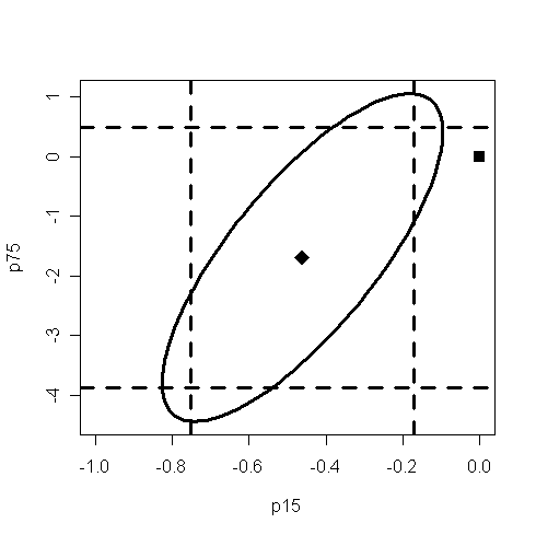
> plot(ellipse(g, c(2,3)), lwd=3, type="l", xlim=c(-1,0))  # the 95% confidence region for p15 and p75. "c(2,3)" appoints the 2nd and the 3rd estimates, i.e., p15 and p75, in the object g. "type" and "xlim" are graphic options. 
> points(0, 0, cex=1.5, pch=15)  # add the point (0,0) to the plot. the "points" command can add points on the plot. "cex" and "pch" are graphic options, use "help(par)" to get more information.
> points(g$coef[2], g$coef[3], cex=2,pch=18) # add the estimates of p15 and p75 to the plot.
> abline(v=c(-0.4612050-2.014103*0.1446425, -0.4612050+2.014103*0.1446425),lwd=3,lty=2) # 95% confidence interval of p15. The "abline" command can add straight lines on the plot.
> abline(h=c(-1.6915757-2.014103*1.0835862, -1.6915757+2.014103*1.0835862),lwd=3,lty=2) # 95% confidence interval of p75.

• Q: What information have you found from the plot? How to interpret the information?

• Note that the estimated values of b_p15 and b_p75 is the center of the ellipse.

• Note that 0 is not in the confidence interval of b_p15. Q: what does it mean?

• Note that 0 is in the confidence interval of b_p75. Q: what does it mean?

• Since the origin (0,0) lie outside the confidence region, we reject the hypothesis that H₀:b_p15=b_p75=0.

  • In some circumstances, the origin (0,0) could lie within both one-way CIs, but lie outside the ellipse. In this case, both one-at-a-time t-tests would not reject the null whereas the joint test would.

  • Q: How to interpret the result if the origin lie outside the rectangle but inside the ellipse?

• Let's find out how the shape of the ellipse is related to two types of correlations.

  > cor(p15, p75) # the correlation between predictors p15 and p75

  [1] -0.9084751

  > summary(g,cor=T)$cor[2,3] # the correlation between estimators of b_p15 and b_p75.

  [1] 0.7653286

  • Q: Check whether it equals the correlation between predictors p15 and p75.

  • Explain why the two correlations are different. How are they related? The two correlations are often different in sign.

    • Loosely speaking, two positively correlated predictors will attemp to perform the same job of explanation. The more work one does, the less the other needs to do, and hence a negative correlation in their estimators of effects. For the negatively correlated predictors, the effect is reversed.

  • Q: Which correlation is directly related to the positive slope of the major axis of the ellipse?

confidence interval for the prediction of mean response

For the model g, let's try to construct a 95% confidence interval for the prediction of mean response at p15=4, p75=3, inc=1100, and gro=3. Q: Check it's an interpolation or an extrapolation.

> x0 <- c(1,4,3,1100,3) # don't forget to include the intercept
> y0 <- sum(x0*g$coef) # the estimate of mean response
> y0 # the average saving when p15=4, p75=3, inc=1100, and gro=3 is 22.5

> qt(0.975, g$df) # the 95% critical value

• Q: Now, how to calculate the standard error of the estimate?

> x <- model.matrix(g) # the model matrix X
> xtxi <- solve(t(x)%*%x) # (X^TX)^-1

> bm <- sqrt(t(x0)%*%xtxi%*%x0) * summary(g)$sigma  # this is the standard error of the estimate of mean response. Q: what does "summary(g)$sigma" estimate?
> bm # take a look of its value

> c(y0-qt(0.975,g$df)*bm, y0+qt(0.975,g$df)*bm) # the 95% confidence interval for the prediction of mean response. confidence interval = estimate ± (critical value)*(s.e. of estimate).

There is a more direct method in R as follows for computing the confidence interval of prediction.
> predict(g, data.frame(p15=4, p75=3,i nc=1100, gro=3), se=T, interval="confidence") # use "help(predict.lm)" to get more information about the command. The "interval="confidence"" option returns the C.I. of mean response whereas "interval="prediction"" returns the C.I. of future observation. Note that the default confidence level is 0.95.

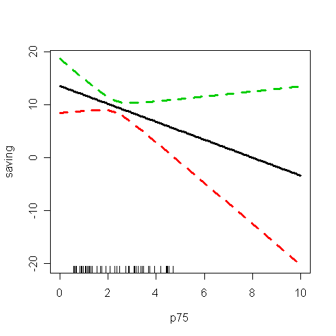
Let us now generate a pointwise confidence band for predictor p75 when other predictors are fixed at their mean values.

> grid <- seq(0, 10, 0.1) # predict mean response at these p75 values

> p <- predict(g, data.frame(p15=mean(p15), p75=grid, inc=mean(inc), gro=mean(gro)), se=T, interval="confidence") # obtain the estimates of mean response and their C.I.'s

> matplot(grid, p$fit, lty=c(1,2,2), lwd=3, type="l", xlab="p75", ylab="saving") # draw the prediction line and confidence band. the "matplot" command plots the columns of one matrix against the columns of another

> rug(p75) # the observed values of p75.

• Q: What information have you found from the plot? How to interpret the information?

• Note that some C.I.'s contain negative values, which is unrealistic because saving should always be no less than zero. This reminds us the danger of extrapolation, i.e., the fitted model may not hold outside the range of p75.

  • In some instances, impossible values in the CI can be avoided by transforming the response, say taking logs, or by using a probability model more appropriate to the response.

  • The normal distribution has supports on the whole real line and so negative values are always possible.

• We see that the confidence bands become wider as we move away from the range of the data.

  • Notice that this widening does not reflect the possibility that the mean structure of the model may change as we move into the region without observed data.

  • The widening only reflect the uncertainty in the parametric estimates, but not uncertainty about the model.

confidence interval for the prediction of future observation

The prediction of future observation has same predicted value as the prediction of mean response. However, the former will have a wider C.I. than the latter because we must take into consideration the variance of e, a future error.

> bmf <- sqrt(1+(t(x0)%*%xtxi%*%x0)) * summary(g)$sigma # compare it with the "bm" above. Note that the 1 comes from future error
> bmf # take a look of the value

> c(y0-qt(0.975,g$df)*bmf, y0+qt(0.975,g$df)*bmf) # the 95% confidence interval for the prediction of future observation. confidence interval = estimate ± (critical value)*(s.e. of estimate).

> predict(g, data.frame(p15=4, p75=3, inc=1100, gro=3), interval="prediction") # a convenient way to obtain the confidence interval. the "interval="prediction"" option returns the C.I. for the prediction of future observation

Compare it with the CI for the prediction of mean response.