Hierarchical or Nested Multinomial Responses (Reading: Faraway (2006), section 5.2)

Consider the data collected by Lowe et al. (1971) concerning live births with deformations of the central nervous system in south Wales. Let us first read the data into R and take a look:

> cns <- read.table("cns.txt")
> cns

In the dataset,

• the variable NoCNS indicates no central nervous system (CNS) malformation

• the variable An denotes anencephalus

• the variable Sp denotes spina bifida

• the variable Other represents other malformations

• the variable Water is water hardness

• subjects are categorized by the type of work performed by the parents (the variable Work)

• Notice that the Area is confounded with the Water

We might consider a multinomial response with the four categories: NoCNS, An, Sp, and Other. However,

• we can see that most births suffer no malformation and so this category dominate the other three

• it is better to consider this as a hierarchical response as in the lecture note

We now separately develop a binomial model for whether malformation occurs and a multinomial model for the type of malformation.

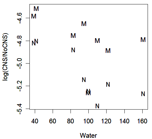
We start with the binomial model. First, we accumulate the number of CNS births and plot the data with the response on the logit scale:

> cns$CNS <- cns$An+cns$Sp+cns$Other
> plot(log(CNS/NoCNS) ~ Water, cns, pch=as.character(Work))

We observe that:

• the proportion of CNS births falls with increasing water hardness

• the proportion of CNS births is higher for manual workers

• one observation (Manual, Newport, Water=100, logit=-5.26) may be an outlier

Because Area is confounded with Water, we cannot put both these predictors in one model. Let us try them both in different models and compare:

> binmodw <- glm(cbind(CNS,NoCNS) ~ Water + Work, cns, family=binomial)

> binmoda <- glm(cbind(CNS,NoCNS) ~ Area + Work, cns, family=binomial)
> anova(binmodw,binmoda,test="Chi")

Notice that:

• if Water is regarded as a nominal variable, it will has the same effect as Area

• therefore, one can view this test as a check for linear trend in the effect of water hardness

• we find that the simpler model using Water is acceptable

• a check for an interaction effect revealed nothing significant (exercise)

• a look at the the residuals is worthwhile:

> halfnorm(residuals(binmodw))



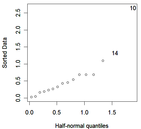
We see an outlier corresponding to Newport manual workers. The case deserves closer examination.

> summary(binmodw)

We see that:

• the residual deviance is close to the degrees of freedom indicating a reasonable fit to the data

• since:

  > exp(-0.3390577)

  [1] 0.7124413

  births to non-manual workers have a 29% lower chance of CNS malformation

• water hardness ranges from about 40 to 160. So, a difference of 120 would decrease the odds of CNS malformation by about 32%:

  > exp(120*(-0.0032644))

  [1] 0.6758879

Now, consider a multinomial model for the three malformation types conditional on a malformation having occurred. As this data is grouped, it is most convenient to present the response as a matrix formed by An, Sp, and Other:

> library(nnet)

> cmmod <- multinom(cbind(An,Sp,Other) ~ Water + Work, cns)

Let us use the AIC criterion to select important effects:

> nmod <- step(cmmod)

We see that:

• the model selection procedure ends up with a model containing only the intercept, i.e., neither predictor has significant effect.

• the fitted model is:

  > summary(nmod, cor=F)

  Call:

  multinom(formula = cbind(An, Sp, Other) ~ 1, data = cns)

   

  Coefficients:

        (Intercept)

  Sp      0.2896333

  Other  -0.9808293

   

  Std. Errors:

        (Intercept)

  Sp     0.08264518

  Other  0.11967839

   

  Residual Deviance: 1374.455

  AIC: 1378.455

• the fitted proportions are:

  > cc <- c(0, 0.2896333, -0.9808293)
  > names(cc) <- c("An","Sp","Other")
  > exp(cc)/sum(exp(cc))

         An        Sp     Other

  0.3688761 0.4927954 0.1383285

So, we find that

• water hardness and parents' profession are related to the probability of a malformed birth

• but, they have no effect on the type of malformation

• if we fit a multinomial logit model to all 4 categories and use NoCNS as the baseline category:

  > amod <- multinom(cbind(NoCNS,An,Sp,Other) ~ Water + Work, cns)

  # weights:  16 (9 variable)

  initial  value 117209.801938

  iter  10 value 27783.394982

  iter  20 value 20770.391437

  iter  30 value 11403.858565

  iter  40 value 5239.204601

  iter  50 value 4716.675652

  final  value 4695.482597

  converged

  Call:

  multinom(formula = cbind(NoCNS, An, Sp, Other) ~ Water + Work,

      data = cns)

   

  Coefficients:

        (Intercept)        Water WorkNonManual

  An      -5.455141 -0.002908840    -0.3638797

  Sp      -5.071047 -0.004323052    -0.2435884

  Other   -6.594670 -0.000513569    -0.6421775

   

  Residual Deviance: 9390.965

  AIC: 9408.965

  We find that

  • both Water and Work are significant (exercise)

  • the fact that Water and Work do not distinguish the type of malformation is not easily discovered from this model