Nominal Multinomial Responses (Reading: Faraway (1st ed., 2006), section 5.1)

Consider a data from the 1996 American National Election Study. Let us first read the data into R and take a look:

> nes96 <- read.table("nes96.txt")
> nes96

For simplicity, we consider only the variables age, educ (education level), and income (income group of the respondents) as the predictors. Our response will be PID (party identification) of the respondents. The original PID involved 7 categories; we will collapse this to three: Democrat, Independent, or Republican, again for simplicity of the presentation. The category Democrat, after collapse, will be regarded as the baseline category.

> sPID <- nes96$PID
> levels(sPID)

> levels(sPID) <- c("Independent", "Independent", "Independent", "Democrat", "Republican", "Democrat", "Republican")
> levels(sPID)

> sPID <- relevel(sPID, ref="Democrat")
> summary(sPID)

The income variable in the original data was an ordered factor with income ranges. We would like to convert this to a numeric variable by taking the midpoint of each range:

> levels(nes96$income)

> inca <- c(115, 10.5, 11.5, 12.5, 13.5, 14.5, 16, 18.5, 21, 23.5, 27.5, 32.5, 37.5, 4, 1.5, 42.5, 47.5, 55, 6, 67.5, 82.5, 8, 97.5, 9.5)
> nincome <- inca[unclass(nes96$income)]
> summary(nincome)

The educ variable is also an ordered factor. The default of R sorts the levels in alphabetical order so that we must re-arrange them according to their natural order:

> levels(nes96$educ)

> nes96$educ <- factor(nes96$educ, levels=c("MS", "HSdrop", "HS", "Coll", "CCdeg", "BAdeg", "MAdeg"))

> levels(nes96$educ)

> summary(nes96$educ)

Let us start with a graphical look at the relationship between the predictors and the response. The response is at the individual level and so we need to group the data just to get a sense of how the party identification is associated with the predictors:

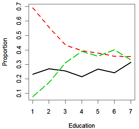
> matplot(prop.table(table(nes96$educ,sPID),1), type="l", xlab="Education", ylab="Proportion", lty=c(1,2,5), lwd=2)

We see that

• the proportion of Democrat (red line) falls with educational status, reaching a plateau for the college educated (level 4 or above)

• the proportion of Republican (black line) rising with educational level and reaching a similar plateau

We cut the income variable into seven levels and use the approximate midpoints of the ranges to label the seven groups:

> cutinc <- cut(nincome,7)
> il <- c(8,26,42,58,74,90,107)
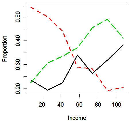
> matplot(il,prop.table(table(cutinc,sPID),1), lty=c(1,2,5), type="l", ylab="Proportion", xlab="Income", lwd=2)

We see that as the income increases,

• the proportion of Republican (black line) and Independent (green line) increases

• the proportion of Democrat (red line) decreases

The age variable is also cut into seven levels and use the approximate midpoints of the ranges to label the groups:
> cutage <- cut(nes96$age,7)
> al <- c(24,34,44,54,65,75,85)
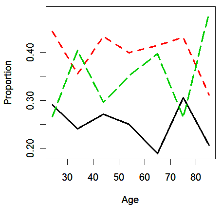
> matplot(al,prop.table(table(cutage,sPID),1), lty=c(1,2,5), type="l", ylab="Proportion", xlab="Age", lwd=2)

We see that the relationship between party identification and age is not clear.

Notice that this is cross-sectional rather than longitudinal data

• so, we cannot say anything about what might happen to an individual with, for example, increasing income

• we can only expect to make conclusions about the relative probability of party affiliations for different individuals with different incomes

We might ask whether the trend we saw in the plots are statistically significant. We will need to model the data to answer this question.

Multinomial Logit Model.

We fit a multinomial logit model using Democrat as the baseline category. The multinom in the nnet package can do the job:

> library(nnet)
> mmod <- multinom(sPID ~ age + educ + nincome, nes96)

The multinom program use the optimization method from the neural net trainer in nnet package to compute the maximum likelihood, but there is no deeper connection to neural networks.

We can select which variables to include the model based on the AIC criterion using a stepwise search method (c.f.: the difference-in-deviance approach for model selection given in previous lab):

> mmodi <- step(mmod)

We see that:

• at the first stage, omitting educ (education) would be the best option to reduce the AIC criterion

• at the next stage, age is removed resulting in a model with only income

• exercise: check whether the model selection result is consistent with the information observed in the 3 plots given above, especially focus on the educ variable

We can also use the standard likelihood method to derive a deviance-based test to compare nested models. For example, we can fit a model without educ and then compare the deviances:

> mmode <- multinom(sPID ~ age + nincome, nes96)

> deviance(mmode) - deviance(mmod)

> mmod$edf-mmode$edf

> pchisq(16.20642, 12, lower=F)

We see that

• educ (education) is not significant relative to the full model. This may seem somewhat surprising given the plot

• however, the large differences between the proportions of Democrat and Republican occur for groups with low education, which represent only a small number of people:

  > (13+52)/sum(summary(nes96$educ))

  [1] 0.06885593

Based on the selected model under the AIC criterion, we can obtain predicted values for specified values of income. For example, suppose we pick the midpoints of the income groups we selected for the earlier plot:

> cbind(il, predict(mmodi,data.frame(nincome=il),type="probs"))

We see that:

• the sum of proportions in same row must equal one

• the probability of being Republican or Independent increases with income (Note: do not give a longitudinal-type conclusion)

• the probability of being Democrat decreases with income

• the default form of R just gives the most probably category:

> predict(mmodi,data.frame(nincome=il))

[1] Democrat   Democrat   Democrat   Republican Republican Republican Republican

Levels: Democrat Independent Republican

　

We may also examine the coefficients to gain an understanding of the relationship between the predictors and the response:

> summary(mmodi, corr=F)

We see that:

• the Democrat category is the baseline category so that we do not find its coefficient in the output

• the intercept terms model the probabilities of the party identification for an income of zero. We can see the relationship from this calculation:

> cc <- c(0, -1.174933, -0.950359)
> exp(cc)/sum(exp(cc))

[1] 0.5898167 0.1821588 0.2280245

The values are the same as:

> predict(mmodi,data.frame(nincome=0),type="probs")

   Democrat Independent  Republican

  0.5898168   0.1821588   0.2280244

• the slope terms represent the log-odds of moving from the baseline category of Democrat to Independent and Republican, respectively, for a unit change of $1000 in in come. We can see more explicitly what this means by predicting probabilities for income $1000 apart and then computing the log-odds:

> (pp <- predict(mmodi,data.frame(nincome=c(0,1)),type="probs"))

   Democrat Independent Republican

1 0.5898168   0.1821588  0.2280244

2 0.5857064   0.1838228  0.2304708

> log(pp[1,1]*pp[2,2]/(pp[1,2]*pp[2,1]))

[1] 0.01608683

> log(pp[1,1]*pp[2,3]/(pp[1,3]*pp[2,1]))

[1] 0.01766457

• log-odds can be difficult to interpret particularly with many predictors and interactions. Sometimes, computing predicted probabilities for a selected range of predictors can provide better intuition

Multinomial Log-Linear Model.

It is possible to fit a multinomial logit model using a Poisson GLM. We can

• declare a factor that has a level for each category of the multinomial response, called response factor;

• declare a factor that has a level for each covariate class in the data, called case factor;

• and then, treat the individual components of the multinomial response as Poisson responses.

We can regard it as a 2-way table with case and response factors as row and column factors, respectively. We set up these variables, also illustrating what happens with the first three multinomial observations:

> sPID[1:3]

> cm <- diag(3)[unclass(sPID),]
> cm[1:3,]

> y <- as.numeric(t(cm))
> y[1:9]

> length(y)

The case factor is:

> case.factor <- gl(944,3)
> case.factor[1:9]

> length(case.factor)

The response factor is:

> res.factor <- gl(3,1,3*944,labels=c("D","I","R"))
> res.factor <- relevel(res.factor, ref="D")

> res.factor[1:9]

> length(res.factor)

We also need to replicate the predictor income:

> rnincome <- rep(nincome, each=3)
Now, examine the form of the reorganized data:

> data.frame(y, case.factor, res.factor, rnincome)[c(1:9),]

Notice that the income variable can be regarded as an effect of the case factor because for the (Poisson) observations with same values of case factor, their income values are identical.

As with the contingency table models, the null model has only main effects of row and column factors:

> nullmod <- glm(y ~ case.factor + res.factor, family=poisson)
> summary(nulmod)

We see that:

• there are 943 effects for the case factor because it has 944 levels, each for a covariate class

• the 943 effects represent the differences between row marginal totals, which is not meaningful in the case

• the model corresponds to a multinomial logit model without any predictors

• the 2 effects of the response factor represent the difference between the 3 party affiliation categories

• the fitted model has a large residual deviance of 2041.3 on 1886 degrees of freedom, which suggests that the probabilities of the three categories are not constant over the predictors

The effect of income is modeled with an interaction with party affiliation:

> glmod <- glm(y ~ case.factor + res.factor + res.factor:rnincome, family=poisson)

> summary(glmod)

We see that:

• the deviance of the model, 1985.4, is the same as the multinomial logit model with income predictor given above

• because only two interaction parameters are identifiable, the last one res.factorR:rnincome, being inestimable, is not estimated.

• the parameterization of the Poisson model is slightly different from the multinomial logit model. The Poisson model makes Republican as the reference level rather than Democrat. We can change it back by:

> res.factorI_rnincome <- model.matrix(glmod)[,948]
> res.factorR_rnincome <- model.matrix(glmod)[,949]
> glmodrD <- glm(y ~ case.factor + res.factor + res.factorI_rnincome + res.factorR_rnincome, family=poisson)
> summary(glmodrD)

Call:

glm(formula = y ~ case.factor + res.factor + res.factorI_rnincome +

    res.factorR_rnincome, family = poisson)

 

Deviance Residuals:

    Min       1Q   Median       3Q      Max 

-1.0804  -0.8050  -0.6985   0.6998   1.3756 

 

Coefficients:

                       Estimate Std. Error   z value Pr(>|z|)   

(Intercept)          -5.385e-01  1.001e+00    -0.538    0.591   

case.factor2         -1.737e-10  1.414e+00 -1.23e-10    1.000   

   ...deleted...

case.factor944       -1.239e+00  1.427e+00    -0.868    0.385   

res.factorI          -1.175e+00  1.536e-01    -7.649 2.03e-14 ***

res.factorR          -9.504e-01  1.417e-01    -6.708 1.98e-11 ***

res.factorI_rnincome  1.609e-02  2.850e-03     5.645 1.65e-08 ***

res.factorR_rnincome  1.766e-02  2.653e-03     6.660 2.75e-11 ***

---

Signif. codes:  0 '***' 0.001 '**' 0.01 '*' 0.05 '.' 0.1 ' ' 1

 

(Dispersion parameter for poisson family taken to be 1)

 

    Null deviance: 2074.2  on 2831  degrees of freedom

Residual deviance: 1985.4  on 1884  degrees of freedom

AIC: 5769.4

 

Number of Fisher Scoring iterations: 6

We find that:

• the Poisson model generates the same coefficients as the multinomial logit model above

• the intercept terms in the multinomial logit model become the main effects of the response factor and the slopes terms become the interactions

• we can get the same results of the multinomial logit model using the Poisson model. In other words, the multinomial logit model can be viewed as a GLM-type model, which allows us to apply all the common methodology developed for GLM