Negative Binomial Response (Reading: Faraway (2006), section 3.3)

For a count response y_x with the property Var(y_x)>>E(y_x), an alternative to the dispersion-parameter approach is to model y_x as negative-binomially distributed, where the negative binomial records the number of "failures" before the r^th "success" in a series of i.i.d. Bernoulli trials (rather than the total number of trials before the r^th success). We will demonstrate the negative-binomial approach using a data from an experiment performed by ATT. The experiment varied five factors relevant to a wave-soldering procedure for mounting components on printed circuit boards. The response variable, skips, is a count of how many solder skips appeared to a visual inspection. The data comes from Comizzoli, Lanwehr, and Sinclair (1990). Let us first read the data into R and take a look at it:

> solder <- read.table("solder.txt")

> solder

    Let us start the analysis by fitting an ordinary Poisson GLM (i.e., s²=1) to the data:

> modp <- glm(skips ~ . , family=poisson, data=solder)
> summary(modp)

Notice that:

• all five factors are significant in this analysis, but

• the model has a residual deviance of 1829 on 882 degrees of freedom, which suggests

  • this is not a good fit

  • the significances of the effects may not be reliable because the standard errors of the estimates of the effects are under-estimated if overdispersion exists

Let us examine whether we can change the Xb structure by including all 2-factor interactions to improve the deviance to an acceptable level:
> modp2 <- glm(skips ~ (Opening +Solder + Mask + PadType + Panel)^2 , family=poisson, data=solder)
> anova(modp,modp2,test="Chi")

The difference-in-deviance test has a very small p-value=9.99e-106, which shows that the model with interactions is a much better fit than the one without interactions. However, let us check whether the new model can pass the goodness-of-fit test:

> deviance(modp2)

> df.residual(modp2)

> pchisq(1068.817,790,lower=FALSE)

Unfortunately,

• it is not enough to conclude that the model fits

• although we can try add more interactions (such as 3-factor interactions), it will make interpretation increasingly difficult

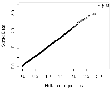
A check for outliers as shown below reveals no problem:

> halfnorm(residuals(modp2))

    Suppose that overdispersion is the cause of large deviance. A negative binomial approach can be adopted. We can specify the value of r (a parameter of negative binomial). Notice that when r is fixed, the model is still an ordinary GLM. Here, we choose r=1 to demonstrate the method under a main-effect model although there is no substantive motivation from this application to use r=1: 

> library(MASS)
> modn <- glm(skips ~ .,negative.binomial(1),solder)
> summary(modn)

We could experiment with different values of r, but there is a more direct way of achieving this by allowing the parameter r to vary and be estimated using maximum likelihood (notice that when r is treated as a parameter, the model is not an ordinary GLM):

> library(MASS)

> modnr <- glm.nb(skips ~ .,solder)

> summary(modnr, cor=F)

We can see that:

• the estimate of r is 4.397 with a standard error of 0.495

• when conditioning on r=4.397, we can use the usual inferential techniques for an ordinary GLM to compare the negative binomial model

• we can compare the result with what obtained from the dispersion-parameter approach as given below:

  > (dp <- sum(residuals(modp,type="pearson")^2)/modp$df.res)

  [1] 2.022422

  > summary(modp,dispersion=dp)

  Call:

  glm(formula = skips ~ ., family = poisson, data = solder)

   

  Deviance Residuals:

      Min       1Q   Median       3Q      Max 

  -3.6413  -1.2562  -0.5286   0.5670   4.7289 

   

  Coefficients:

              Estimate Std. Error z value Pr(>|z|)   

  (Intercept) -1.10042    0.13179  -8.350  < 2e-16 ***

  OpeningM     0.57161    0.08115   7.044 1.87e-12 ***

  OpeningS     1.81475    0.07173  25.301  < 2e-16 ***

  SolderThin   0.84682    0.04731  17.898  < 2e-16 ***

  MaskA3       0.51315    0.10094   5.084 3.70e-07 ***

  MaskA6       1.81103    0.09398  19.270  < 2e-16 ***

  MaskB3       1.20225    0.09523  12.624  < 2e-16 ***

  MaskB6       1.86648    0.08974  20.800  < 2e-16 ***

  PadTypeD6   -0.40328    0.08573  -4.704 2.55e-06 ***

  PadTypeD7   -0.08979    0.07851  -1.144 0.252753   

  PadTypeL4    0.22460    0.07277   3.086 0.002026 **

  PadTypeL6   -0.70633    0.09439  -7.483 7.26e-14 ***

  PadTypeL7   -0.48260    0.08783  -5.495 3.91e-08 ***

  PadTypeL8   -0.30778    0.08336  -3.692 0.000222 ***

  PadTypeL9   -0.63793    0.09228  -6.913 4.74e-12 ***

  PadTypeW4   -0.19021    0.08065  -2.358 0.018349 * 

  PadTypeW9   -1.56252    0.13034 -11.988  < 2e-16 ***

  Panel        0.14670    0.02482   5.910 3.42e-09 ***

  ---

  Signif. codes:  0 '***' 0.001 '**' 0.01 '*' 0.05 '.' 0.1 ' ' 1

   

  (Dispersion parameter for poisson family taken to be 2.022422)

   

      Null deviance: 8788.2  on 899  degrees of freedom

  Residual deviance: 1829.0  on 882  degrees of freedom

  AIC: 3967.6

   

  Number of Fisher Scoring iterations: 5

  Exercise: examine what is different and what is similar between the results from the negative-binomial and the dispersion-parameter approaches