Rate Models (Reading: Faraway (2006), section 3.2)

Purott and Reeder (1976) presented some data from an experiment conducted to determine the effect of gamma radiation on the number of chromosomal abnormalities (ca) observed. The number of cells exposed in each run (cells, in hundreds) differs. The dose amount (doseamt) and the rate (doserate) at which the dose is applied are the predictors of interest. Let us read the data into R and take a look at it:

> dicentric <- read.table("dicentric.txt")

> dicentric

Notice that:

• we can model the response as binomially distributed, i.e., y_x~binomial(100n_x, p_x), where y_x is ca and n_x is cells, and use appropriate link function and Xb structure to relate p_x to the predictors. In other words, we can apply a binomial GLM to the data.

• because the values of y_x/(100n_x) are small (its maximum value is 1.43/100=0.0143) as shown in the table below and the values of 100n_x are relatively large, a Poisson approximation to the binomial is effective, i.e., a Poisson GLM is an effective alternative for the data

• however, because the values of n_x differs, it does not make much sense to build a Poisson GLM using ca as the response and doseamt and doserate as the predictors (Q: how to interpret the value of prediction if we fit such a model?)

• therefore, n_x, which is the size variable in this case, should play a role in the Poisson GLM so that meaningful conclusions can be drawn

Let us take a look at how the proportions, y_x/n_x, change with the two predictors:
> round(xtabs(ca/cells ~ doseamt+doserate, dicentric),2)

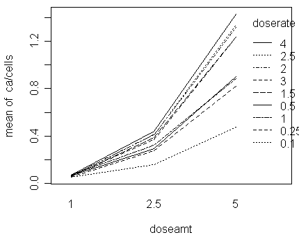
We can see that:

• the proportion increases with doserate and doseamt

• the effect of doserate seems larger than doseamt

• furthermore, the effect of doserate is not linear

  • its influence could be multiplicative, i.e., doserate influences ca/cells through multiplication rather than addition

  • a log transformation can sometimes simplify a multiplicative model

  • exercise: draw some scatter plots to check whether the relationship between ca/cells and log(doserate) is more linear

  • we will replace doserate by log(doserate) in the following analysis

• it is clear that some interaction effects are significant

  • however, if we replace ca/cells by log(ca/cells), the interactions can possibly be reduced (or even removed in some cases) (Q: can you see why?)

  • because log[y_x/(100n_x)]»logit[y_x/(100n_x)] when y_x/(100n_x) is small, we can expect that the result of fitting a Normal linear model to log(ca/cells) would be similar to that of fitting a binomial GLM with logit link to ca

  • exercise: use a Normal linear model to relate the response log(ca/cells) to the predictors and give your opinions on its pro's and con's

• an interaction plot can offer a good visual summary of the 4 points given above:

  > with(dicentric,interaction.plot(doseamt,doserate,ca/cells))

  

    Let us treat log(doserate) as a continuous variable and dosamt as a categorical variable and fit a Normal linear model to the response ca/cells:

• Q: why dosamt treated as categorical?

• notice that dosamt has 3 levels and  its effect on ca/cells cannot be explained only by a linear effect as shown in the interaction plot. Therefore, no matter we use the linear-quadratic coding or the dummy-variable coding, the two effects coded from dosamt would be both significant and span the same column space

• on the other hand, log(doserate) has 9 levels but its effect on ca/cells seems only linear. If we use the dummy-variable coding, it will require 7 more degrees of freedom to explain the difference between levels

> dicentric$dosef <- factor(dicentric$doseamt)

> lmod <- lm(ca/cells ~ log(doserate)*dosef, dicentric)
> summary(lmod)

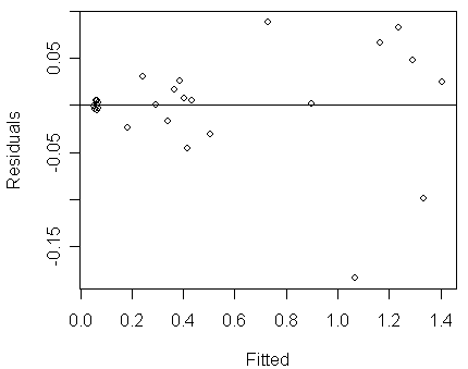
As can be seen from the R², the model fits well. However, a look at the diagnostics reveals a problem:
> plot(residuals(lmod) ~ fitted(lmod),xlab="Fitted",ylab="Residuals")
> abline(h=0)

Notice that:

• we can see clear evidence of non-constant variance (Var(y_x) increases with E(y_x)).

• we might prefer an approach that directly model the count response, say ca~Poisson. However, the size variable n_x should be appropriately included in the model so that its effect can be correctly adjusted for

    Let us consider the Poisson model, y_x~Poisson(m_x), with the link function:

        log(m_x/n_x)=h_x=Xb    Û    log(m_x)=log(n_x)+Xbºh_x'.

The log(n_x) is now regarded as a predictor with the coefficient fixed as one. In this manner, we are modeling the rate of chromosomal abnormalities while still maintaining the count response for the Poisson model. In R, we can fix the coefficient as one by using an offset, which is a term on the predictor side with no parameter attached:

> rmod <- glm(ca ~ offset(log(cells))+log(doserate)*dosef, family=poisson,dicentric)
> summary(rmod)

Notice that:

• from the residual deviance, the model fits well

• given the significant interaction effects, we can see that the linear effect of log(doserate) is different depending on the level of doseamt

  • its linear effect, or slope, is 0.07178 for doseamt=1, 0.07178+0.16122=0.233 for doseamt=2.5, and 0.07178+0.19350=0.26528 for doseamt=5. The slopes increase with doseamt.

  • Q: if we use linear-quadratic coding for doseamt, we would expect that the linear-by-linear and linear-by-quadratic interactions between log(doserate) and doseamt would be significant. How can you interpret the significance of the two interactions? Compare it with the previous interpretation for interactions coded based on dummy variables. Which interpretation is easier to understand for you?  

  • the combination of a high doseamt and a high doserate has a greater combined effect than the main effect estimates would suggest.

• exercise: fit a binomial GLM with logit link to the data and compare its result with this Poisson fitted model

Suppose that we are not sure whether it is reasonable to set the coefficient of log(n_x) as one. We can allow a parameter for the predictor as follows:

        log(m_x)=g×log(n_x)+Xbºh_x'    Û    log(m_x/n_x^g)=h_x=Xb.

This is a Poisson GLM with log(n_x) as an ordinary predictor:

> pmod <- glm(ca ~ log(cells)+log(doserate)*dosef, family=poisson,dicentric)
> summary(pmod)

Notice that:

• the estimated g, 1.00252, is very close to one, which supports the use of the previous Poisson model

• not surprisingly, the estimated b are only slightly different from the previous Poisson fitted model