Poisson Regression (Reading: Faraway (2006), section 3.1)

    Here is a data which recorded the counts of the numbers of species of tortoise found on 30 Galapagos Islands and the numbers that are endemic to that island. The data also contains five geographic variables for each island. The data was presented by Johnson and Raven (1973). A few missing values that appeared in the original dataset have been filled for simplicity. We start the analysis of the data by reading the data into R and throw out the Endemics variable (which falls in the 2nd column of the data frame) since we won't be using it in this analysis.
> gala <- read.table("gala.txt")

> gala

> gala <- gala[,-2]

    Let us first fit a Normal linear model:

> modl <- lm(Species ~ . , gala)
> summary(modl)

We find that:

• the fit has a fairly good R², 76.58%, which seems suggest this is a good fit.

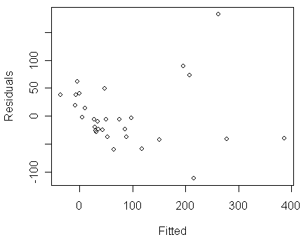
• however, let us take a look at a diagnostic plot of residuals versus fitted values:

> plot(predict(modl),residuals(modl),xlab="Fitted",ylab="Residuals")

Notice that:

• in the figure, we can see clear evidence of non-constant variance (i.e., Var(y_x) becomes larger when E(y_x) increases)

• Q: for the distributions we have ever seen in the lectures, which one has the property that its variance increases with its mean?

• Q: why all points lie above a downward sloping line on the left side of the figure? It happens because

  1. the values of the response ³ a constant c, which is 0 in this case, and

  2. many values of the response » c (which can be found from the stem plot below)

  Because of 1., residual = y-(fitted y) ³ c-(fitted y). Because of 2., many residuals » c-(fitted y), which accounts for the line forming a lower bound on the scatter plot of residual versus fitted y. 

  > stem(gala$Spec) 

    The decimal point is 2 digit(s) to the right of the |

   

    0 | 0000111122223344

    0 | 566679

    1 | 001

    1 |

    2 | 4

    2 | 89

    3 |

    3 | 5

    4 | 4

• if we persist in the Normal linear model approach, a possible remedy is to transform the response. Some experimentation (such as the use of the Box-Cox transformation method) suggests that a square-root transformation is best

Let us follow the suggestion to fit a model by using the square-root of Species as the response and draw the same residual plot for the new model:

> modt <- lm(sqrt(Species) ~ . , gala)

> plot(predict(modt),residuals(modt),xlab="Fitted",ylab="Residuals")

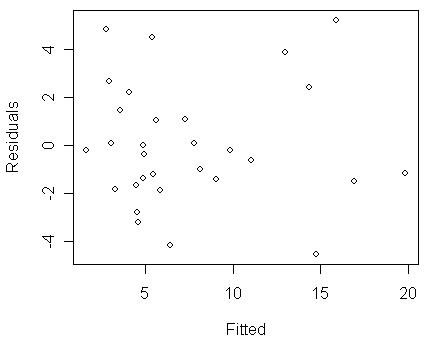
We now see that the non-constant variance problem have been cleared up in the new model. Let us take a look at the fit:

> summary(modt)

Notice that:

• we see a fairly good fit (R²=0.7827) considering the nature of the variables

• however, we achieved this fit at the cost of transforming the response

• the transformation makes interpretation more difficult because the estimated parameters need to be interpreted with respect to the scale of square-root of count 

• for this data, some of the response values are quite small and close to the lower bound of count (i.e., 0), which makes us question the validity of the a Normal linear model

    For count responses as in this case, we can model the response by using Poisson distribution. Notice that the variance of Poisson increases with its mean. We now fit a Poisson GLM to the Galapagos data:
> modp <- glm(Species ~ .,family=poisson,gala)
> summary(modp)

The format of the output is same as that for binomial GLM because they are members of generalized linear models. We can find from the output that:

• the residual deviance is 716.85 on 24 degrees of freedom, which indicates an ill-fitting model if the Poisson is the correct model for the response (i.e., the null hypothesis). Some explanations for the large deviance are:

  • outlier

  • wrong Xb structure

  • over-dispersion

  We will examine the validity of these explanations in the following analysis.

• exercise: compare the results of this Poisson GLM fit and the Normal linear model fits. Check what information in the two results are similar, what are different. Explain why Nearest, and Scruz are so significant in the Poisson fit, but insignificant in the Normal fits. What could possibly cause it?

Using the function written by Prof. Faraway, we can draw a half-normal plot for the residuals to see whether the large deviance can be explained by an outlier:

> halfnorm(residuals(modp))

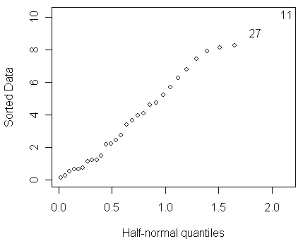
We do not see any clear evidence of outlier in the half-normal plot.

It could be the Xb structure form of the model needs some improvement, but some experimentation with different form for the predictors will reveal that :

• there is little scope for improvement (exercise: perform different Xb structures to confirm it by yourself)

• furthermore, the proportion of deviance explained by this model, i.e., 1-716.85/3510.73=0.7958117, is about the same as the R² in the Normal linear model above

Let us now go to the last explanation --- over-dispersion. For a Poisson distribution, the mean is equal to the variance. Let us investigate this relationship for this model. It is difficult to estimated the variance for a given value of the mean, but (y_x-(m_x-hat))² does serve as a crude approximation. We plot this estimated variance against the mean:

> plot(log(fitted(modp)),log((gala$Species-fitted(modp))^2),xlab=expression(hat(mu)),ylab=expression((y-hat(mu))^2))
> abline(0,1)

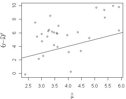
We see that the variance is proportional to, but larger than, the mean.

    For the cases of over-dispersion, we can generalize the Poisson GLM by allowing a dispersion parameter s² such that:

        Var(y_x)=s²E(y_x).

The dispersion parameter can be estimated by:

> (dp <- sum(residuals(modp,type="pearson")^2)/modp$df.res)

We can then adjust the standard errors of b-hat and so forth in the summary as follow:

> summary(modp,dispersion=dp)

Notice that:

• the estimation of the dispersion parameter s² and the regression parameter b are independent, so choosing a dispersion other than one has no effect on the regression parameter estimation (exercise: check whether the two Poisson fits, with and without dispersion parameter, have same estimates of b)

• but, the standard errors and z-statistics are changed

• exercise: compare this result with the Normal linear model fits. Examine what information in the results are similar, what are different. (Notice that  Nearest and Scruz become insignificant in the Poisson fit with dispersion parameter, which is consistent with what we observed in the Normal fits.)

To compare two nested models, we now need to use F-test, rather than chi-square test:

> drop1(modp,test="F")

The F-test is more reliable than the z-statistics although it makes little difference for this data.