Overdispersion (Reading: Faraway (2006, 1st ed.), section 2.11)

Manly (1978) reported a data from an experiment where boxes of trout eggs were buried at five different stream locations and retrieved at four different times. The times are specified by the number of weeks after the original placement. The number of surviving eggs was recorded. Let us first read the data into R and construct a tabulation of the data:

> troutegg <- read.table("troutegg.txt")

> ftable(xtabs(cbind(survive,total) ~ location+period, troutegg))

Notice that

• in one case, all the eggs survive, while in another, none of the eggs survive

• therefore, we would expect that within the range of the predictors in the dataset, the true p_x can run from 0 to 1, which indicates:

  • a Normal linear model with y_x/n_x as the response should not be a good approximation to the binomial model

  • the choice of link functions could be an important issue for this case

We can obtain the survival proportion in each cell by:

> xtabs((survive/total) ~ location+period, troutegg)

We can find some rough conclusions from the table:

• no matter what length of retrieving time is chosen, location 5 has a survival probability much lower than other locations

• the survival probabilities in the other 4 locations are more consistent

• it seems that the survival probabilityhas the tendency of decreasing over retrieving time

• it is not clear whether there exists some strong interactions between location and period   

    Let us fit a binomial GLM with only main effects to the data. We now treat location and period as nominal variables although period can be regarded as a quantitative variable:

> troutegg$location <- as.factor(troutegg$location)

> troutegg$period <- as.factor(troutegg$period)

> bmod <- glm(cbind(survive,total-survive) ~ location + period, family=binomial,troutegg)

> summary(bmod)

Notice that the deviance of 64.495 on 12 degrees of freedom shows that this model does not fit. Some possible causes of the large deviance are:

• sparse data

• outlier

• wrong Xb structure (the current model only contains main effects)

• overdispersion

Before we conclude that there is an overdispersion, we need to eliminate other potential explanations.

    With about 100 eggs in each box, we have no problem with sparseness.

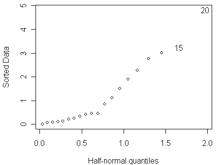
    To check for outliers, a half-normal plot of the residuals is a good way. Here is a function for drawing half-normal plot written by Prof. Faraway:

> halfnorm(residuals(bmod))

From the half-normal plot, we find that:

• no single outlier is apparent

• perhaps one can discern a larger number of residuals which seem to follow a more dispersed distribution than the rest.

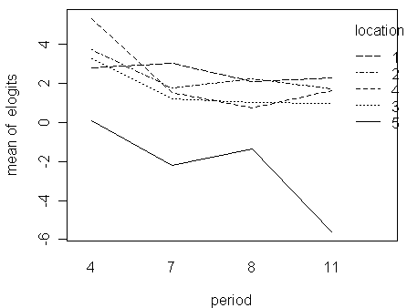
    For the Xb structure, we can add the 3´4=12 interaction effects to the current main-effect model. After doing this, the new model is a saturated model so that its deviance is zero. In other words, the deviance decreases by 64.495 for 12 degrees of freedom, which of course is statistically significant in terms of the difference-in-deviance test. However, let us draw an interaction plot by using as the response the empirical logits, which can be regarded as empirical estimates of h_x=logit(p_x) and are defined as:

        log[(y_x+0.5)/(n_x-y_x+0.5)].

The 0.5 are added to prevent infinite values when n_x=y_x.

> elogits <- log((troutegg$survive+0.5)/(troutegg$total-troutegg$survive+0.5))
> with(troutegg,interaction.plot(period,location,elogits))

Notice that:

• interaction plots are always difficult to interpret conclusively

• for this case, we can say the five lines are roughly parallel to each other if the sharp decrease in the end of the location-5 line is ignored; in other words, there is no obvious sign of large interactions

• we might conclude that although interactions are statistically significant, they are not physically very significant

• so, there is no clear evidence that the Xb structure with only main effects is inadequate

    Having eliminated these more obvious causes of large deviance, we may put the blame on overdispersion. Possible reasons for the overdispersion include:

• heterogeneous trout eggs

• variation in the experimental procedures

• unknown variables affecting survival probability

• ...

The simplest approach for modeling overdispersion is to introduce an additional dispersion parameter s². We can estimate the dispersion parameter as:

> (sigma2 <- sum(residuals(bmod,type="pearson")^2)/12)

We see that this is substantially larger than one as it would be in the standard binomial GLM.

    We can now make F-test (c.f., chi-square test for standard binomial GLM) on the predictors using:

> drop1(bmod,scale=sigma2,test="F")

Notice that:

• both predictors are significant (note: we can see from the interaction plots that some main effects can be removed to further simplify the model)

• in the command, it is necessary to specify the scale argument using the estimated value of s²

• if this  scale argument is omitted, the deviance, rather than Pearson X², will be used in the estimation of s²

  • this makes very little difference in this particular dataset

  • but, in some cases, using the deviance instead of Pearson X² to estimate s² gives inconsistent results

• the warning message reminds us that the use of s² results in a model that is no longer a standard binomial GLM

• no goodness-of-fit test is possible because we now have a free dispersion parameter s²

    To test the significance of individual parameters, we can use the estimated s² to scale up the standard errors of parameter estimates:

> summary(bmod,dispersion=sigma2)

(exercise:

1. compare the results with the output of the standard binomial GLM

2. find their differences

3. explain how the differences affect the conclusions.)

(Q: should we still use Normal(0,1) to calculate the p-values? is t-distribution a better choice?)