Estimation Problem (Reading: Faraway (2006, 1st ed.), section 2.8)
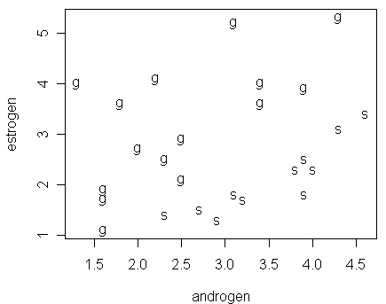
Margolese (1970) reported a data that recorded urinary androsterone (androgen) and etiocholanolone (estrogen) values from 26 healthy males. Among them, 15 men are homosexual (labeled as "g" in the orientation variable) and 11 heterosexual (labeled as "s"). We start by reading the data into R and drawing a plot of it:
>
hormone <- read.table("hormone.txt")
> hormone
androgen estrogen orientation
1 3.9 1.8 s
2 4.0 2.3 s
3 3.8 2.3 s
…deleted…
26 1.3 4.0 g
> plot(estrogen ~ androgen,data=hormone,pch=as.character(orientation))

Notice that:
it seems possible to draw a clear-cut line in the figure to separate the two groups of men
this is an example of "sparse data," i.e., data with small nx (nx=1 in this case)
Q: for sparse data, what analysis results of binomial GLM will become less reliable?
We now fit a binomial GLM to see if the orientation can be predicted from the two hormone values:
> modl <- glm(orientation ~ estrogen + androgen, hormone, family=binomial)
Warning messages:
1: algorithm did not converge in: glm.fit(x = X, y = Y, weights = weights, start = start, etastart = etastart,
2: fitted probabilities numerically 0 or 1 occurred in: glm.fit(x = X, y = Y, weights = weights, start = start, etastart = etastart,
Notice that:
when yx is a Bernoulli response (i.e, yx=0 or 1), we can put yx directly as the response variable in the glm function. There is no need to form another column that contains 1-yx
as shown in the warning message, there were problems with the convergence of the algorithm used to approximate MLE
A look at the summary reveals further evidence:
> summary(modl)
Call:
glm(formula = orientation ~ estrogen + androgen, family = binomial, data = hormone)
Deviance Residuals:
Min 1Q Median 3Q Max
-2.759e-05 -2.107e-08 -2.107e-08 2.107e-08 3.380e-05
Coefficients:
Estimate Std. Error z value Pr(>|z|)
(Intercept) -84.49 136095.03 -0.001 1
estrogen -90.22 75910.98 -0.001 1
androgen 100.91 92755.62 0.001 1
(Dispersion parameter for binomial family taken to be 1)
Null deviance: 3.5426e+01 on 25 degrees of freedom
Residual deviance: 2.3229e-09 on 23 degrees of freedom
AIC: 6
Number of Fisher Scoring iterations: 25
Notice that
the residual deviance is extremely small, which indicates that this is a very good fit
however, chi-square goodness-of-fit test may not be accurate because of sparseness
none of the predictors are significant under the Wald test; the insignificance is caused by their high standard errors
two possible explanations of the high standard error: linearly separable property existing in the dataset as will be explained below and sparseness
note: for sparse data, the standard errors may be overestimated Þ this is known as the Hauck-Donner effect Þ deviance-based test is preferred (see its results in the next command)
the maximum default number of iterations (25) has been reached but the algorithm had not converged
it implies the current estimated values of b are not reliable
note: the convergence problem is caused by the linearly separable property, rather than sparseness
Let us now perform deviance-based method to test the significance of individual parameters:
> drop1(modl,test="Chi")
Single term deletions
Model:
orientation ~ estrogen + androgen
Df Deviance AIC LRT Pr(Chi)
<none> 2.323e-09 6.000
estrogen 1 27.437 31.437 27.437 1.623e-07 ***
androgen 1 28.257 32.257 28.257 1.062e-07 ***
---
Signif. codes: 0 '***' 0.001 '**' 0.01 '*' 0.05 '.' 0.1 ' ' 1
Notice that:
both predictors have significant contribution to the reduction of deviance
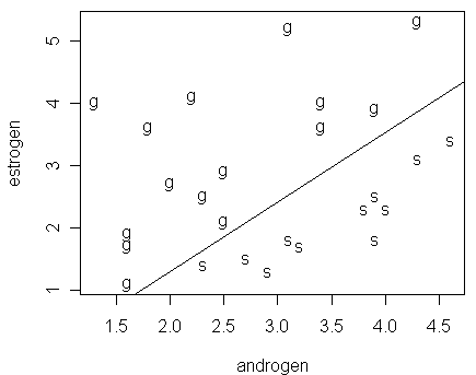
the deviance-based test reveals the information we would expect from the next figure --- both estrogen and androgen are now significant
remember that for sparse data, the test involving differences of deviances is more accurate than the goodness-of-fit test involving only a single deviance
We now go back to the problem of unstable parameter estimation. Let us take a look at a figure, which computes the line corresponding to px=1/2, where px is predicted using the fitted model modl. The figure reveals the reason for the instability in parameter estimation:
> abline(-84.49/90.22,100.91/90.22)

Notice that:
the two groups are linearly separable so that a perfect fit is possible
for the data, we suffer from an "embarrassment of riches" --- a perfect fit is achievable (Þ suggest that perfect predictions could be possible), but the estimates of the parameters and their standard errors are unstable
Let us try to estimate the parameters by using a bias-reduction method proposed by Firth (1993). The estimates have the advantage of always being finite:
>
library(brglm)
>
modb <- brglm(orientation ~ estrogen + androgen, hormone, family=binomial)
>
summary(modb)
Call:
brglm(formula = orientation ~ estrogen + androgen, family = binomial,
    data = hormone)


Coefficients:
            Estimate Std. Error z value Pr(>|z|)
(Intercept)  -3.6502     2.9104 -1.2542  0.20976
estrogen     -3.5853     1.4985 -2.3926  0.01673 *
androgen      4.0732     1.6206  2.5134  0.01196 *
---
Signif. codes:  0 ‘***’ 0.001 ‘**’ 0.01 ‘*’ 0.05 ‘.’ 0.1 ‘ ’ 1

(Dispersion parameter for binomial family taken to be 1)

    Null deviance: 28.92309  on 25  degrees of freedom
Residual deviance:  3.70078  on 23  degrees of freedom
Penalized deviance: 4.18374
AIC:  9.70078
Notice that:
the estimates obtained from the bias-reduction method are quite different from that in the glm result
under the bias-reduction method, the two predictors are significant (because their t-values are quite extreme compared with a t-distribution with 23 degrees of freedom), which we expect given the previous figure
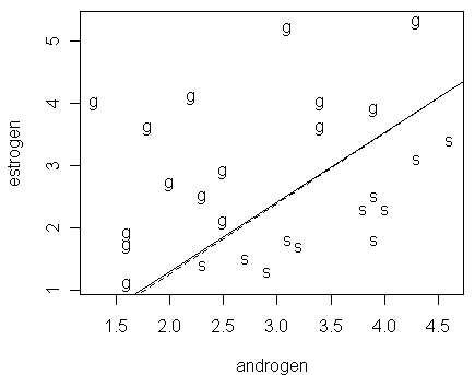
By using the fitted model in the brglm result, we add the line corresponding to px=1/2:
> abline(-3.6502/3.5853,4.0732/3.5853,lty=2)

Notice that:
although the fit from the brglm command appears to be different from the glm result (judging from their estimated values of parameters), their fitted probabilities are effectively very close as we can see from the figure
whether the data is effective depends on the purpose of analysis
for prediction or classification purpose, this is a good dataset, but
it is not so useful for the purpose of parameter estimation