Choice of Link Function (Reading: Faraway (2006, 1st ed.), section 2.7)
Bliss (1935) analyzed some data on the number of insects dying at different levels of insecticide concentration. Let us first read into R the data and take a look of it:
>
bliss <- read.table("bliss.txt")
>
bliss
dead alive conc
1 2 28 0
2 8 22 1
3 15 15 2
4 23 7 3
5 27 3 4
ˇ@
We now fit the binomial GLM to the data under the three link functions --- logit, probit, and complementary log-log:
>
modl <- glm(cbind(dead,alive) ~ conc, family=binomial, data=bliss)
>
modp <- glm(cbind(dead,alive) ~ conc, family=binomial(link=probit), data=bliss)
>
modc <- glm(cbind(dead,alive) ~ conc, family=binomial(link=cloglog), data=bliss)
ˇ@
We start by considering the fitted values of probability px:
> fitted(modl) # or use the command "predict(modl,type="response")"
1 2 3 4 5
0.08917177 0.23832314 0.50000000 0.76167686 0.91082823
An alternative way to obtain these values is to use linear predictor, hx:
> coef(modl)[1]+coef(modl)[2]*bliss$conc
[1] -2.323790e+00 -1.161895e+00 4.440892e-16 1.161895e+00 2.323790e+00
The values of linear predictor can also be obtained from:
> modl$linear.predictors # or use the command "predict(modl)"
1 2 3 4 5
-2.323790e+00 -1.161895e+00 4.440892e-16 1.161895e+00 2.323790e+00
The fitted values of probability are then:
> ilogit(modl$linear.predictors)
1 2 3 4 5
0.08917177 0.23832314 0.50000000 0.76167686 0.91082823
Notice the need to distinguish between predictions in the scale of the response (i.e., px) and the link (i.e., hx).
ˇ@
Now, let us compare the logit, probit, and complementary log-log fits:
> cbind(fitted(modl),fitted(modp),fitted(modc))
[,1] [,2] [,3]
1 0.08917177 0.08424186 0.1272700
2 0.23832314 0.24487335 0.2496909
3 0.50000000 0.49827210 0.4545910
4 0.76167686 0.75239612 0.7217655
5 0.91082823 0.91441122 0.9327715
These are not very different, but now look at a wider range -2<concentration<8:
>
x <- seq(-2,8,0.2)
>
pl <- ilogit(modl$coef[1]+modl$coef[2]*x)
>
pp <- pnorm(modp$coef[1]+modp$coef[2]*x)
>
pc <- 1-exp(-exp((modc$coef[1]+modc$coef[2]*x)))
>
plot(x,pl,type="l",ylab="Probability",xlab="Dose")
>
lines(x,pp,lty=3)
>
lines(x,pc,lty=5)

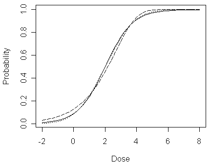
In the figure, logit fit is shown by a solid line, probit fit a dotted line, complementary log-log a dashed line. We can see that:
when 0.2 < px <0.8, the three lines do not seem very different (both on their differences and on their ratios)
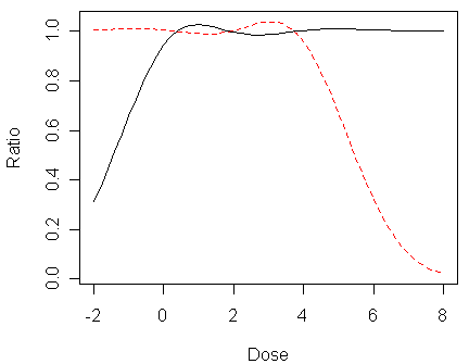
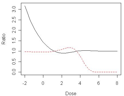
however, when px is close to 0 or 1, although their differences are still small, their ratios differ substantially as shown in the following two figures
This is problematic since the concentration in the dataset falls in the range: [0, 4], which indicates it would be difficult to distinguish between these link functions using the data
> matplot(x,cbind(pp/pl,(1-pp)/(1-pl)),type="l",xlab="Dose",ylab="Ratio")

In the figure, the lower tail ratio of probit to logit probabilities (i.e., px,probit/px,logit) is given by the solid line, the upper tail ratio (i.e., (1-px,probit)/(1-px,logit)) is given by the dashed line.
> matplot(x,cbind(pc/pl,(1-pc)/(1-pl)),type="l",xlab="Dose",ylab="Ratio")

In the figure, the lower tail ratio of complementary log-log to logit probabilities is given by the solid line, the upper tail ratio is given by the dashed line.