>
2+3 # R can be used as a simple calculator
> exp(1)
# All the usual calculator functions are available
> pnorm(1.645)
# the normal probability function
The assignment operator is "<-"
>
x <- 2
# assign the value 2 to x
> y <- 3
# y is 3
> z <- x+y
# assign the sum to z
> z
# look at the result
Vector and matrix valued variables are also possible. The c(), cbind() and rbind() functions are useful for building these up.
>
x <- c(1,9,7,3)
# x is a length 4 vector
> x
# take a look
[1] 1 9 7 3
> y <- 1:4
# ":" is useful for assigning a sequence
> y
# take a look
[1] 1 2 3 4
> z <- x+y # vector arithmetic works as expected
> z
# take a look
[1] 2 11 10 7
> xm <- cbind(x,y,z)
# make a matrix by binding x, y, z together column-wise
> xm # take a look
x y z
[1,] 1 1 2
[2,] 9 2 11
[3,] 7 3 10
[4,] 3 4 7
> t(xm)
# the transpose of xm
[,1] [,2] [,3] [,4]
x 1 9 7
3
y 1 2 3
4
z 2 11 10 7
> rbind(x, y, z) # make a matrix by binding x, y, z together
row-wise
[,1] [,2] [,3] [,4]
x 1 9 7
3
y 1 2 3
4
z 2 11 10 7
Now let's look at getting some simple statistics:
>
x <- rnorm(50)
# generat 50 standard normal random numbers
> mean(x)
# the mean
> var(x)
# the variance
> summary(x)
# 5 number summary plus the mean
Min. 1st Qu. Median
Mean 3rd Qu. Max.
-1.95200 -0.57150 0.19750 0.06371 0.76080 2.35200
> stem(x) # a stemplot of x
The decimal point is at the |
-2 | 0
-1 | 96
-1 | 42110
-0 | 9877665
-0 | 443221
0 | 0022223344444
0 | 5578888899
1 | 334
1 | 5
2 | 04
>
y <- rnorm(50)
# more random numbers
> cor(x,y)
# the correlation of x and y
Now, let's do some nice graphics:
>
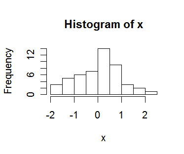
hist(x) # a histogram of x

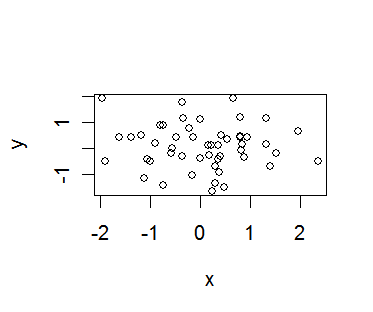
> plot(x,y) # a simple scatter plot

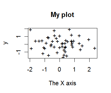
> plot(x,y,pch="+",xlab="The X axis",main="My plot")
# add some more options to the plot

To find out more online use the "help()" command:
>
help(cbind)
# If you know the command you want help for
Lets see how we enter data into R.
Here is a data
set for test. You can save it as a text file to a directory, say "c:/mydata/",
with a file name, say "gala.data".
> gala <- read.table("c:/mydata/gala.data")
# read the data into R
Or, you can change the working directory to "c:/mydata" (do this by
choosing "檔案"->"變更現行目錄",
and then inputting the directory name). And now you can simply read
the data into R by:
>
gala <- read.table("gala.data")
# read the data into R
> gala
# take a look
Species Endemics Area Elevation Nearest
Scruz Adjacent
Baltra 58
23 25.09 346
0.6 0.6 1.84
Bartolome 31
21 1.24 109
0.6 26.3 572.33
Caldwell 3
3 0.21 114
2.8 58.7 0.78
... stuff deleted ...
Wolf 21 12 2.85 253 34.1 254.7 2.33
R stores whole datasets in dataframes. It's a convenient way of keeping all the variables together.
> dim(gala)
# check the dimension of the data
[1] 30 7
You can select a variable from the data by:
> gala$Species # pick out a particular variable
[1] 58 31 3 25 2
18 24 10 8 2 97 93 58 5 40 347 51 2 104
[20] 108 12 70 280 237 444 62 285 44 16 21
>
gala$Sp # unique abbreviations work
[1] 58 31 3 25
2 18 24 10 8 2 97 93 58 5 40 347 51 2 104
[20] 108 12 70 280 237 444 62 285 44 16 21
> attach(gala)
# makes the prepending of gala unnecessary - see next line
> Species
[1] 58 31 3 25
2 18 24 10 8 2 97 93 58 5 40 347 51 2 104
[20] 108 12 70 280 237 444 62 285 44 16 21
You can select a subset of the data by:
> gala[2,]
# the second row
> gala[,3] # the third
column
> gala[2,3] # the (2,3)
element
> gala[c(1,2,4), ] # the first,
second, and fourth rows
> gala[3:6,] # the third
through sixth rows
> gala[,-c(1,2)] # "-" indicates
"everything but", this keeps all data except the first two columns
Area Elevation Nearest Scruz Adjacent
Baltra 25.09 346
0.6 0.6 1.84
Bartolome 1.24 109
0.6 26.3 572.33
... stuff deleted ...
Wolf 2.85
253 34.1 254.7 2.33
> gala[gala$Sp > 300,] #
select those cases whose Species are greater than 300
Species Endemics Area Elevation
Nearest Scruz Adjacent
Isabela 347
89 4669.32 1707
0.7 28.1 634.49
SantaCruz 444
95 903.82 864
0.6 0.0 0.52
More details on R can be found here, here, or here.
The software RStudio provides a better integrated development environment than R does. You can download the free version of RStudio from here (Note that you need to install R before using RStudio).